Create maps from SITG files with sf and ggplot2

TL;DR

In this post, we see how to create a map in R using the sf and ggplot2 package, starting from freely available SHAPE files.

Introduction

In Geneva (Switzerland), we are lucky to have SITG, a website with tons of geographical open datasets. I wanted to try my hand at doing maps in R for some time now, but could not find a way that felt integrated with the other packages I usually work with. Importing .sh files was a challenge (for me), as well as plotting the data in ggplot2 rather than with a dedicated map library like tmap.

All that changed with sf, a package that implements Simple Features for R. Full disclaimer: I know nothing about geographic information systems. All I can say is: if you are already using the tidyverse, sf makes it really straightforward to convert geographical datasets to data.frames/tibbles that you can then manipulate with your usual toolbox (dplyr, tidyr…). To learn more about the ecosystem of R packages for geocomputation, you could do worse than start here.

As I walked around Geneva countryside, I stumbled upon a point of view with several information boards. One showed a little map that I thought would make a good first example.

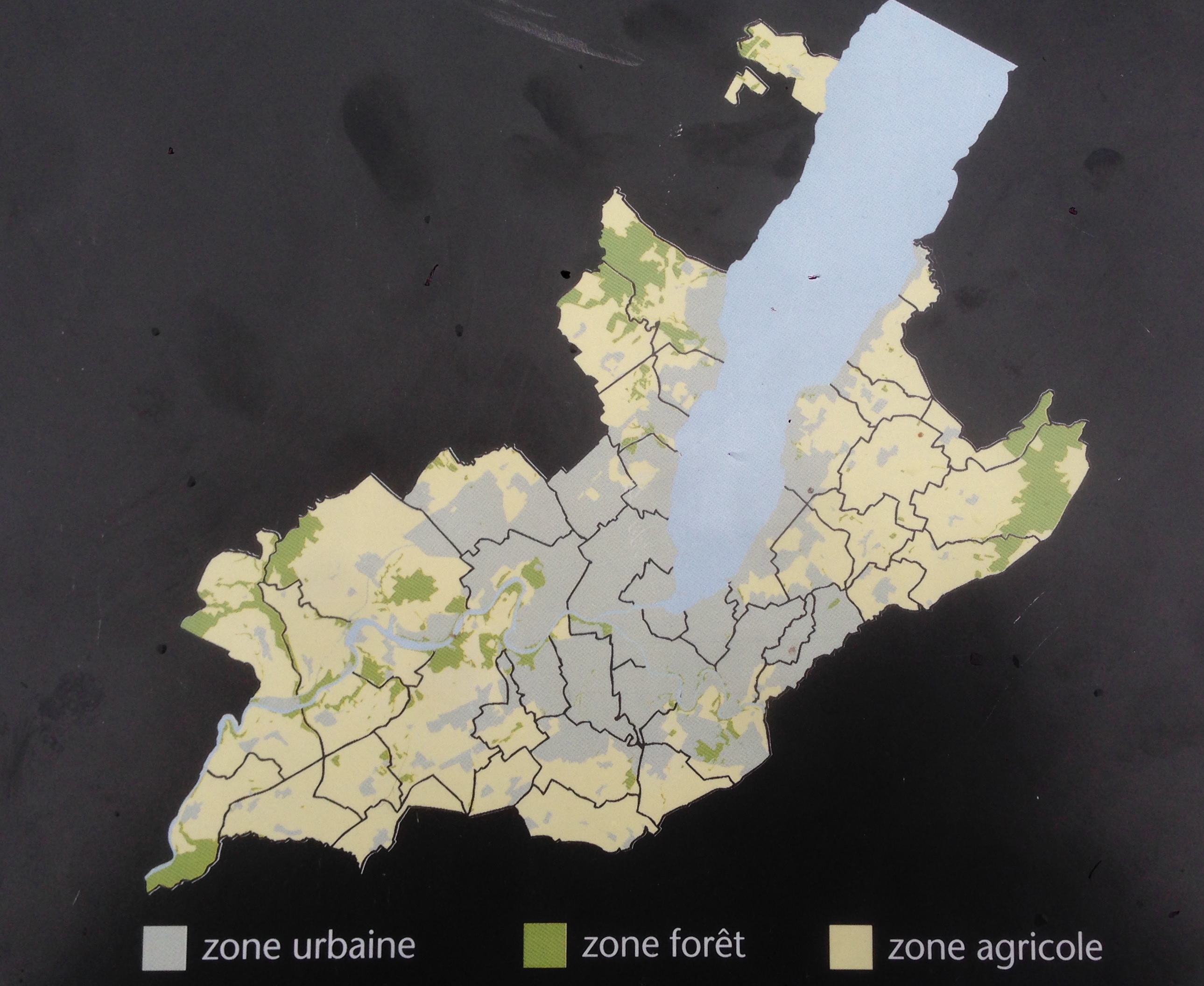
Land use in Geneva, Switzerland

Installing sf

If you already have all dependencies, it might be as straightforward as installing the package sf. On Ubuntu, it was a bit of a pain, especially because I did not read the instructions first. After adding libpng-dev on top of the other libraries, the sf install worked in RStudio.

Planning the map

Thinking in layers - like always with ggplot2 - it looks like we need the following things: 1. borders of each communal districts in Geneva 2. borders of water (lake and main rivers) 3. areas of buildings 4. areas of forests 5. areas of agricultural fields

Mapping communal districts

The polygons of all Geneva communal districts are available here, named ‘COMMUNES GENEVOISES (GEOMETRIE SIMPLIFIEE)’)“. I downloaded the SHP version. Make sure you place all the files (not just the .shp and .shx) in the same directory..shp and .shx are enough to get the polygones, but you would miss all the metadata (like the names of the communes). Using sf function st_read, we can import them into R.

# Load sf and dplyr quietly
suppressMessages(library(sf))
suppressMessages(library(dplyr))

# Load the communes dataset
communes  <- st_read("../data/GEO_COMMUNES_GE_SIMPLIFIEES.shp")

## Reading layer `GEO_COMMUNES_GE_SIMPLIFIEES' from data source `/home/xadam/dev/GitHub/ii_src/content/data/GEO_COMMUNES_GE_SIMPLIFIEES.shp' using driver `ESRI Shapefile'
## Simple feature collection with 48 features and 7 fields
## geometry type:  MULTIPOLYGON
## dimension:      XY
## bbox:           xmin: 2485410 ymin: 1109645 xmax: 2512974 ymax: 1135578
## epsg (SRID):    NA
## proj4string:    +proj=somerc +lat_0=46.95240555555556 +lon_0=7.439583333333333 +k_0=1 +x_0=2600000 +y_0=1200000 +ellps=bessel +units=m +no_defs

We can see that the file was successfully loaded, and that we have 48 geometry (of type MULTIPOLYGON) with 7 columns.

Our usual dataframe functions (dim, names…) work on the sf object. With glimpse from dplyr, we can get a sense of what each column contains (e.g COMMUNE has the names of communes).

# a glimpse at the column content
glimpse(communes)

## Observations: 48
## Variables: 8
## $ COMMUNE    <fctr> Corsier, Carouge, Puplinge, Perly-Certoux, Genève-...
## $ NO_COMM    <int> 19, 8, 39, 35, 22, 21, 28, 13, 41, 7, 29, 47, 33, 2...
## $ ABREVIATIO <fctr> Cr, Ca, Pu, P.C., E.V., V.G., He, C.Bg, Sy, Bx, Ju...
## $ NO_COM_FED <int> 6619, 6608, 6636, 6632, 6621, 6621, 6625, 6613, 663...
## $ LIEN_WWW   <fctr> http://www.geneve-communes.ch, http://www.geneve-c...
## $ SHAPE_AREA <dbl> 2735462, 2703700, 2669651, 2542247, 2538140, 252017...
## $ SHAPE_LEN  <dbl> 8817.079, 8682.215, 8290.230, 7353.972, 7805.008, 8...
## $ geometry   <simple_feature> MULTIPOLYGON (((2506472.244..., MULTIPOL...

The dplyr verbs are also available. So you can filter, rename, mutate… and always get back a sf object.

# Filter to see only commune "Carouge"
communes %>% filter(COMMUNE == "Carouge") %>% head

## Simple feature collection with 1 feature and 7 fields
## geometry type:  MULTIPOLYGON
## dimension:      XY
## bbox:           xmin: 2498785 ymin: 1113794 xmax: 2500854 ymax: 1116325
## epsg (SRID):    NA
## proj4string:    +proj=somerc +lat_0=46.95240555555556 +lon_0=7.439583333333333 +k_0=1 +x_0=2600000 +y_0=1200000 +ellps=bessel +units=m +no_defs
##   COMMUNE NO_COMM ABREVIATIO NO_COM_FED                      LIEN_WWW
## 1 Carouge       8         Ca       6608 http://www.geneve-communes.ch
##   SHAPE_AREA SHAPE_LEN                       geometry
## 1    2703700  8682.215 MULTIPOLYGON (((2499509.292...

# Filter to see only communes with "Genève" in their name
communes %>% filter(grepl("^genève", COMMUNE, ignore.case=T)) %>% head

## Simple feature collection with 4 features and 7 fields
## geometry type:  MULTIPOLYGON
## dimension:      XY
## bbox:           xmin: 2497477 ymin: 1114844 xmax: 2502538 ymax: 1120889
## epsg (SRID):    NA
## proj4string:    +proj=somerc +lat_0=46.95240555555556 +lon_0=7.439583333333333 +k_0=1 +x_0=2600000 +y_0=1200000 +ellps=bessel +units=m +no_defs
##                 COMMUNE NO_COMM ABREVIATIO NO_COM_FED
## 1     Genève-Eaux-Vives      22       E.V.       6621
## 2           Genève-Cité      21       V.G.       6621
## 3 Genève-Petit-Saconnex      23        P.S       6621
## 4    Genève-Plainpalais      24        Pl.       6621
##                        LIEN_WWW SHAPE_AREA SHAPE_LEN
## 1 http://www.geneve-communes.ch    2538140  7805.008
## 2 http://www.geneve-communes.ch    2520179  8975.992
## 3 http://www.geneve-communes.ch    6233939 13848.284
## 4 http://www.geneve-communes.ch    4628296 14154.933
##                         geometry
## 1 MULTIPOLYGON (((2502293.896...
## 2 MULTIPOLYGON (((2499898.226...
## 3 MULTIPOLYGON (((2499654.219...
## 4 MULTIPOLYGON (((2499714.537...

# Select only COMMUNE column (note that geometry is kept)
# I also had to use select.sf rather than the generic select
communes %>% select.sf(COMMUNE) %>% head

## Simple feature collection with 6 features and 1 field
## geometry type:  MULTIPOLYGON
## dimension:      XY
## bbox:           xmin: 2494595 ymin: 1111735 xmax: 2508349 ymax: 1125219
## epsg (SRID):    NA
## proj4string:    +proj=somerc +lat_0=46.95240555555556 +lon_0=7.439583333333333 +k_0=1 +x_0=2600000 +y_0=1200000 +ellps=bessel +units=m +no_defs
##             COMMUNE                       geometry
## 1           Corsier MULTIPOLYGON (((2506472.244...
## 2           Carouge MULTIPOLYGON (((2499509.292...
## 3          Puplinge MULTIPOLYGON (((2507415.896...
## 4     Perly-Certoux MULTIPOLYGON (((2496407.883...
## 5 Genève-Eaux-Vives MULTIPOLYGON (((2502293.896...
## 6       Genève-Cité MULTIPOLYGON (((2499898.226...

# Mutate names to lowercase
communes %>% 
  mutate(COMMUNE = stringr::str_to_lower(COMMUNE)) %>% 
  head

## Simple feature collection with 6 features and 7 fields
## geometry type:  MULTIPOLYGON
## dimension:      XY
## bbox:           xmin: 2494595 ymin: 1111735 xmax: 2508349 ymax: 1125219
## epsg (SRID):    NA
## proj4string:    +proj=somerc +lat_0=46.95240555555556 +lon_0=7.439583333333333 +k_0=1 +x_0=2600000 +y_0=1200000 +ellps=bessel +units=m +no_defs
##             COMMUNE NO_COMM ABREVIATIO NO_COM_FED
## 1           corsier      19         Cr       6619
## 2           carouge       8         Ca       6608
## 3          puplinge      39         Pu       6636
## 4     perly-certoux      35       P.C.       6632
## 5 genève-eaux-vives      22       E.V.       6621
## 6       genève-cité      21       V.G.       6621
##                        LIEN_WWW SHAPE_AREA SHAPE_LEN
## 1 http://www.geneve-communes.ch    2735462  8817.079
## 2 http://www.geneve-communes.ch    2703700  8682.215
## 3 http://www.geneve-communes.ch    2669651  8290.230
## 4 http://www.geneve-communes.ch    2542247  7353.972
## 5 http://www.geneve-communes.ch    2538140  7805.008
## 6 http://www.geneve-communes.ch    2520179  8975.992
##                         geometry
## 1 MULTIPOLYGON (((2506472.244...
## 2 MULTIPOLYGON (((2499509.292...
## 3 MULTIPOLYGON (((2507415.896...
## 4 MULTIPOLYGON (((2496407.883...
## 5 MULTIPOLYGON (((2502293.896...
## 6 MULTIPOLYGON (((2499898.226...

To learn more about applying dplyr verbs to sf objects, see this article from the documentation and Strimas blog post.

To map the polygons, there is now a dedicated geom geom_sf in ggplot2. This makes mapping geo areas as simple as lines (geom_line) or points (geom_point). Note that, at this stage, you need the development version of ggplot2.

# if you don't have the development version
# install.packages("devtools")
# devtools::install_github("tidyverse/ggplot2")
library(ggplot2)

# Create a plot
ggplot() + 
  # add a layer with lightgrey communal polygons
  geom_sf(data=communes) + 
  # add a title
  labs(title="Communals districts of Geneva")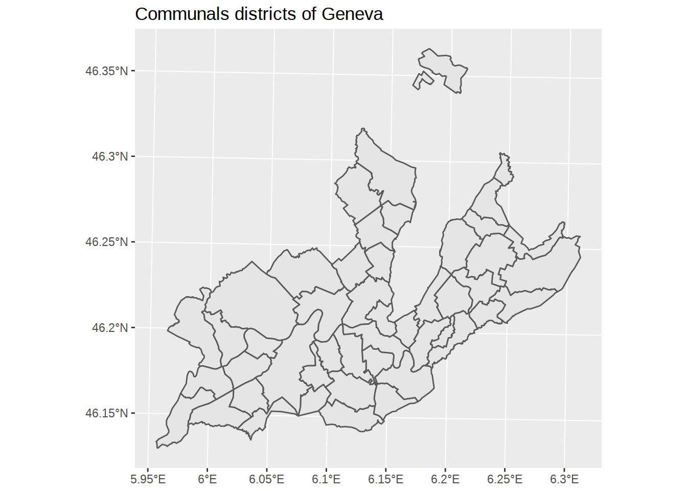

geom_sf accepts styling arguments: fill for the color inside the polygons, color for the color of the polygons borders.

ggplot() + 
  geom_sf(data=communes, fill="darkred", color="gold") + 
  labs(title="Communals districts of Geneva")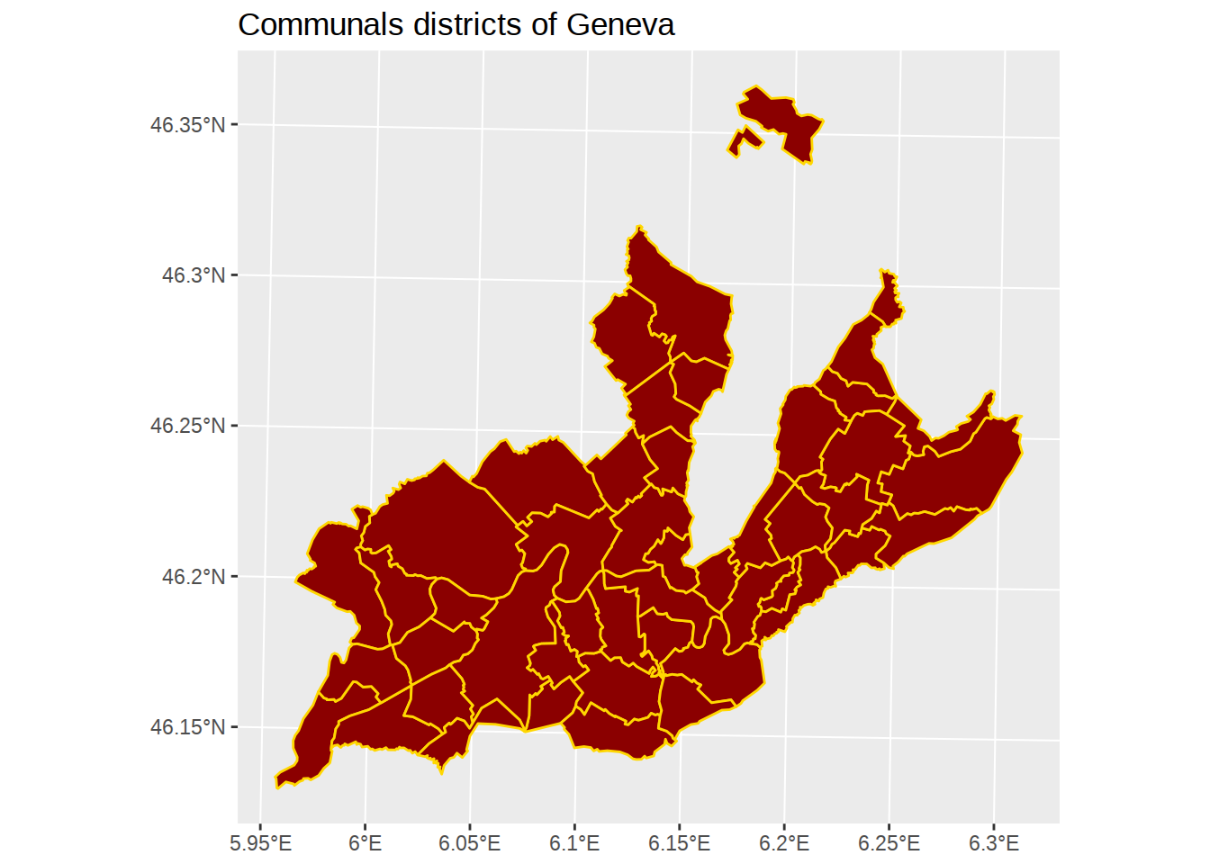

Great! But here we notice something surprising: districts don’t overlap the lake, but they do overlap the rivers. Let’see how we can fix this.

Removing rivers

The polygons of Geneva lake and main rivers (Rhône and Arve) are available here, named ‘EMPRISE DU LAC LEMAN (Petit-lac)’. We can load them with st_read again.

waters <- st_read("../data/GEO_LAC.shp")

## Reading layer `GEO_LAC' from data source `/home/xadam/dev/GitHub/ii_src/content/data/GEO_LAC.shp' using driver `ESRI Shapefile'
## Simple feature collection with 3 features and 3 fields
## geometry type:  POLYGON
## dimension:      XY
## bbox:           xmin: 2485388 ymin: 1110037 xmax: 2510891 ymax: 1136120
## epsg (SRID):    NA
## proj4string:    +proj=somerc +lat_0=46.95240555555556 +lon_0=7.439583333333333 +k_0=1 +x_0=2600000 +y_0=1200000 +ellps=bessel +units=m +no_defs

glimpse(waters)

## Observations: 3
## Variables: 4
## $ NOM        <fctr> Léman, Arve, Rhône
## $ SHAPE_AREA <dbl> 67916036.2, 638356.6, 3148365.7
## $ SHAPE_LEN  <dbl> 64418.43, 21388.25, 59438.90
## $ geometry   <simple_feature> POLYGON ((2510891.1652 1134..., POLYGON ...

There are only 3 geometries: Léman (the lake), Arve and Rhône (the main rivers). Let’s see what they looks like:

# Create a plot
ggplot() + 
  # add a layer with blue water polygons
  geom_sf(data=waters) + 
  # add a title
  labs(title="Lake and rivers of Geneva")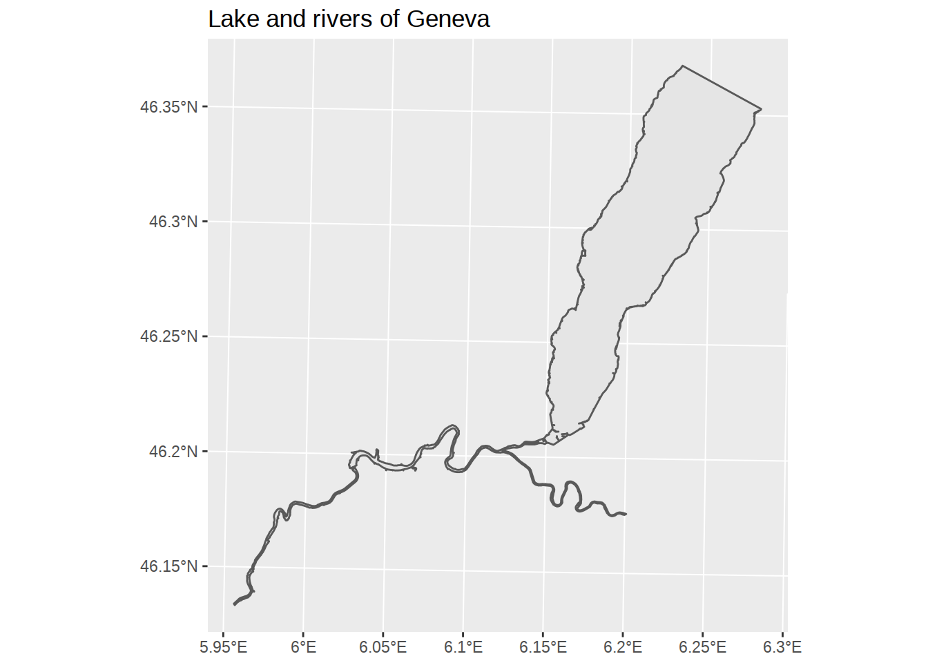

Using dplyr again, let’s filter to see only the rivers.

# Create a plot
ggplot() + 
  # add a layer with blue water polygons
  geom_sf(data= waters %>% filter(NOM != "Léman")) + 
  # add a title
  labs(title="Lake and rivers of Geneva")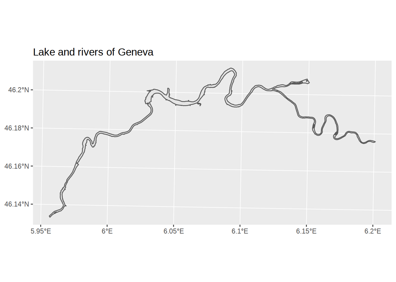

We could map waters on top of the communes. But we could also explore geometry calculations and remove it from the commune shapes. The sf package has functions to combine polygon sets into new sf object. The functions are described in this vignette. You can do things like union (st_union), intersection (st_intersection), difference (st_difference)… Here we will calculate the difference, which keeps everything but the intersection.

Note that we need to “group” the rivers, otherwise nothing will be removed since communes are never overlapped by both rivers in the same place. Below we apply:

st_combine to combine the two rivers in waters to a single multipolygon
st_union to convert the st_combine multipolygon to a normal polygon
st_difference to remove the st_union polygon from communes

communes_no_water <- 
  communes %>%
    st_difference(st_union(st_combine(waters)))

## Warning: attribute variables are assumed to be spatially constant
## throughout all geometries

ggplot() +
  geom_sf(data=communes_no_water) +
  labs(title="Communes without rivers")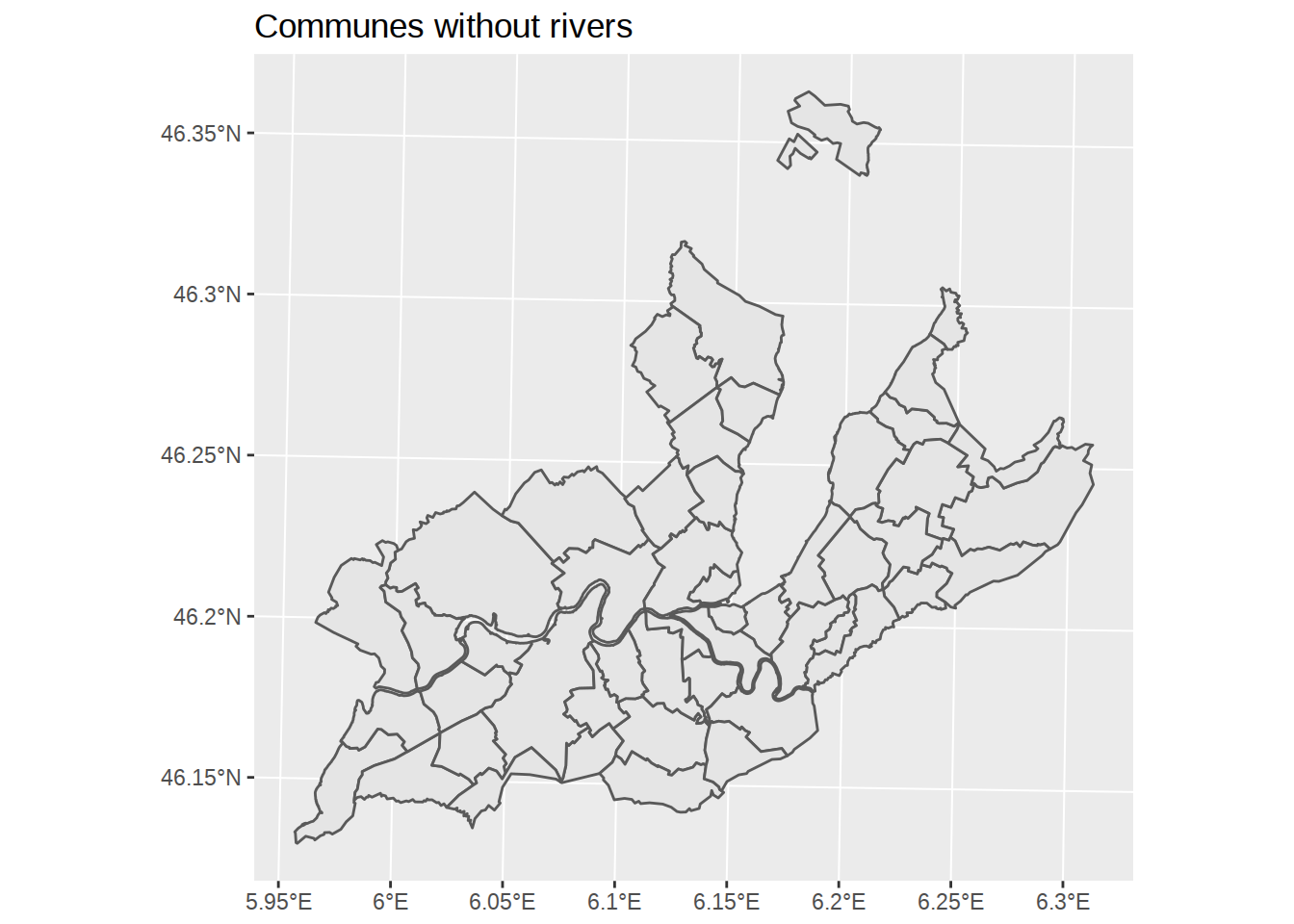

Zoom on the map

To check that rivers were correctly removed, we might want to “zoom” on the map. Playing with coordinates isn’t something I understand well at all. It looks like along geom_sf, a dedicated coordinate function coord_sf was added to ggplot2, which lets us restrict coordinates. However, using limits in the axis unit (like ylim(c(46.2,46.25))) won’t work. Even if latitude and longitude are displayed in this format on the axis, that’s not the format of the undelying data. Let’s see what the coordinates for the first polygon look like:

communes_no_water %>%
  select(geometry) %>%
  slice(1) %>%
  as.character()

## [1] "list(list(list(c(2506472.2448, 2506542.9965, 2506716.5846, 2507240.2961, 2507493.079, 2507486.3281, 2507585.1196, 2507576.499, 2507646.5101, 2507913.8754, 2508176.8697, 2508334.7441, 2508348.9038, 2508268.3703, 2507973.44, 2507700.1959, 2507160.6547, 2507087.6019, 2506884.1048, 2506780.5705, 2506656.0346, 2506420.4294, 2506474.8647, 2506235.2632, 2506251.3018, 2506172.348, 2506198.9391, 2506112.8363, 2506054.4852, 2505828.127, 2505536.5367, 2505536.4371, 2505262.7578, 2505257.80583182, 2505262.7578, \n2505264.218, 2505271.1583, 2505277.1085, 2505291.8989, 2505300.2949, 2505300.3665, 2505300.4338, 2505300.5055, 2505300.5467, 2505300.5774, 2505300.586, 2505300.6495, 2505300.7212, 2505300.793, 2505300.865, 2505300.9245, 2505300.9363, 2505300.957, 2505301.0081, 2505301.0792, 2505301.1511, 2505301.1983, 2505301.2226, 2505301.2596, 2505301.2991, 2505301.3656, 2505301.4368, 2505301.4683, 2505301.5081, 2505301.5792, 2505301.6249, 2505301.6505, 2505301.7218, 2505301.7592, 2505301.7927, 2505301.8456, 2505301.8639, \n2505301.9265, 2505301.9349, 2505302.006, 2505302.0762, 2505302.1476, 2505302.167, 2505302.2187, 2505302.2785, 2505302.2893, 2505302.3279, 2505302.36, 2505302.4164, 2505302.4306, 2505302.5012, 2505302.5719, 2505302.6423, 2505302.7128, 2505302.7677, 2505302.7831, 2505302.8536, 2505302.8709, 2505302.9242, 2505302.9941, 2505303.039, 2505303.0643, 2505303.1344, 2505303.2048, 2505303.2313, 2505303.2747, 2505303.3447, 2505303.415, 2505303.4846, 2505303.5545, 2505303.6233, 2505303.6942, 2505303.7205, 2505303.7638, \n2505303.8335, 2505303.8745, 2505303.9031, 2505303.9164, 2505303.9728, 2505303.9962, 2505304.0423, 2505304.1117, 2505304.1342, 2505304.1812, 2505304.2505, 2505304.2584, 2505304.3198, 2505304.3892, 2505304.4583, 2505304.5275, 2505304.5553, 2505304.5966, 2505304.6309, 2505304.6658, 2505304.7348, 2505304.7966, 2505304.8037, 2505304.8182, 2505304.8397, 2505304.8756, 2505304.9418, 2505304.9933, 2505305.0104, 2505305.0289, 2505305.0793, 2505305.1478, 2505305.1931, 2505305.2165, 2505305.2534, 2505305.2852, \n2505305.305, 2505305.3537, 2505305.3739, 2505305.4222, 2505305.4457, 2505305.4907, 2505305.5176, 2505305.5591, 2505305.6195, 2505305.688, 2505305.7561, 2505305.7964, 2505305.8243, 2505305.8612, 2505305.8926, 2505305.9606, 2505306.0288, 2505306.0817, 2505306.0967, 2505306.1647, 2505306.2202, 2505306.2325, 2505306.2757, 2505306.3005, 2505306.3683, 2505306.419, 2505306.4362, 2505306.5037, 2505306.551, 2505306.5715, 2505306.6391, 2505306.7068, 2505306.7742, 2505306.8417, 2505306.9091, 2505306.9763, 2505307.0437, \n2505307.1118, 2505307.1782, 2505307.2453, 2505307.3123, 2505307.3794, 2505307.4465, 2505307.5134, 2505307.5802, 2505307.6472, 2505307.7139, 2505307.7212, 2505307.7807, 2505307.8473, 2505307.8643, 2505307.9139, 2505307.9805, 2505308.0471, 2505308.1135, 2505308.135, 2505308.1799, 2505308.2464, 2505308.3127, 2505308.379, 2505308.4453, 2505308.5114, 2505308.5775, 2505308.6436, 2505308.7096, 2505308.7755, 2505308.8078, 2505308.8414, 2505308.8792, 2505308.9072, 2505308.973, 2505309.0388, 2505309.0752, \n2505309.1045, 2505309.1465, 2505309.1701, 2505309.236, 2505309.3013, 2505309.3667, 2505309.4323, 2505309.4976, 2505309.563, 2505309.6169, 2505309.6283, 2505309.6934, 2505309.7394, 2505309.7586, 2505309.8238, 2505309.8889, 2505309.9292, 2505309.9541, 2505309.9979, 2505310.0187, 2505310.0837, 2505310.1486, 2505310.2134, 2505310.2772, 2505310.3429, 2505310.3639, 2505310.4075, 2505310.4721, 2505310.5283, 2505310.5367, 2505310.6011, 2505310.6112, 2505310.6655, 2505310.7212, 2505310.73, 2505310.7772, 2505310.7899, \n2505310.8547, 2505310.9133, 2505310.9362, 2505310.9584, 2505310.9839, 2505311.0477, 2505311.1119, 2505311.1718, 2505311.2399, 2505311.2694, 2505311.3037, 2505311.3131, 2505311.3674, 2505311.4015, 2505311.4311, 2505311.4861, 2505311.4947, 2505311.5204, 2505311.5581, 2505311.6201, 2505311.6846, 2505311.7475, 2505311.7629, 2505311.8106, 2505311.8733, 2505311.9364, 2505311.9987, 2505312.0613, 2505312.1236, 2505312.1863, 2505312.2484, 2505312.3102, 2505312.3723, 2505312.4048, 2505312.434, 2505312.485, \n2505312.4958, 2505312.5573, 2505312.6189, 2505312.6323, 2505312.6803, 2505312.7077, 2505312.7415, 2505312.7526, 2505312.8028, 2505312.8281, 2505312.8638, 2505312.9062, 2505312.9248, 2505312.9738, 2505312.9857, 2505313.0466, 2505313.107, 2505313.1185, 2505313.1675, 2505313.1942, 2505313.2278, 2505313.2705, 2505313.2882, 2505313.3124, 2505313.3482, 2505313.3926, 2505313.4083, 2505313.4395, 2505313.4682, 2505313.4844, 2505313.5279, 2505313.5569, 2505313.5877, 2505313.606, 2505313.6473, 2505313.7066, \n2505313.7661, 2505313.8254, 2505313.8844, 2505313.8963, 2505313.9434, 2505313.9629, 2505314.0023, 2505314.0611, 2505314.102, 2505314.1198, 2505314.1783, 2505314.2366, 2505314.2638, 2505314.2951, 2505314.3156, 2505314.3582, 2505314.4113, 2505314.4622, 2505314.4692, 2505314.4759, 2505314.5272, 2505314.5623, 2505314.5848, 2505314.6409, 2505314.7, 2505314.7127, 2505314.7574, 2505314.7858, 2505314.8146, 2505314.8717, 2505314.9202, 2505314.9288, 2505314.9529, 2505314.9857, 2505315.0424, 2505315.0991, 2505315.1559, \n2505315.2021, 2505315.2121, 2505315.2611, 2505315.2684, 2505315.3246, 2505315.3702, 2505315.3807, 2505315.3986, 2505315.4484, 2505315.4601, 2505315.5034, 2505315.516, 2505315.5562, 2505315.5649, 2505315.5717, 2505315.6272, 2505315.6653, 2505315.6827, 2505315.7065, 2505315.7379, 2505315.7904, 2505315.844, 2505315.854, 2505315.9033, 2505315.9402, 2505315.9581, 2505316.0127, 2505316.0351, 2505316.0617, 2505316.0674, 2505316.0783, 2505316.1219, 2505316.1339, 2505316.1762, 2505316.2042, 2505316.2305, \n2505316.2846, 2505316.2999, 2505316.3296, 2505316.3435, 2505316.3925, 2505316.4041, 2505316.4462, 2505316.4999, 2505316.5394, 2505316.5534, 2505316.6071, 2505316.6602, 2505316.666, 2505316.7133, 2505316.7372, 2505316.7635, 2505316.8193, 2505316.8552, 2505316.872, 2505316.9258, 2505316.9603, 2505316.9773, 2505317.0228, 2505317.0298, 2505317.082, 2505317.1342, 2505317.1733, 2505317.1863, 2505317.2382, 2505317.271, 2505317.2901, 2505317.3173, 2505317.3418, 2505317.3935, 2505317.4448, 2505317.486, 2505317.4961, \n2505317.5473, 2505317.5707, 2505317.5985, 2505317.6187, 2505317.6494, 2505317.7003, 2505317.7509, 2505317.7918, 2505317.8016, 2505317.8101, 2505317.852, 2505317.882, 2505317.9023, 2505317.9181, 2505317.9526, 2505317.993, 2505318.0028, 2505318.0123, 2505318.0527, 2505318.1024, 2505318.1356, 2505318.1523, 2505318.17, 2505318.2018, 2505318.2514, 2505318.3006, 2505318.3499, 2505318.3837, 2505318.3991, 2505318.4098, 2505318.4481, 2505318.4656, 2505318.4969, 2505318.5288, 2505318.5456, 2505318.5943, 2505318.6427, \n2505318.6675, 2505318.6911, 2505318.7393, 2505318.7874, 2505318.8181, 2505318.8355, 2505318.8772, 2505318.887, 2505318.9309, 2505318.9785, 2505318.9968, 2505319.026, 2505319.0574, 2505319.0735, 2505319.0974, 2505319.1207, 2505319.1566, 2505319.1679, 2505319.1793, 2505319.2148, 2505319.2463, 2505319.2616, 2505319.2804, 2505319.3084, 2505319.3223, 2505319.3549, 2505319.4013, 2505319.4478, 2505319.491, 2505319.5402, 2505319.5861, 2505319.5955, 2505319.6302, 2505319.6433, 2505319.6505, 2505325.5705, \n2505324.4206, 2505322.65473884, 2505336.3311, 2505344.68364709, 2505346.5114, 2505351.1517, 2505362.4121, 2505363.1322, 2505374.5442, 2505375.9931, 2505387.7857, 2505421.8947, 2505427.8349, 2505433.3353, 2505454.6961, 2505459.4263, 2505463.3165, 2505466.2366, 2505468.5967, 2505479.30271796, 2505490.2176, 2505497.51739588, 2505498.9881, 2505504.0683, 2505528.1592, 2505525.2092, 2505527.6093, 2505535.0498, 2505535.6398, 2505538.4797, 2505539.7499, 2505557.6007, 2505561.7609, 2505569.1513, 2505573.9215, \n2505572.5014, 2505575.2615, 2505576.7216, 2505578.7916, 2505585.9422, 2505588.6622, 2505587.8222, 2505591.0938, 2505592.1423, 2505593.0611, 2505593.1461, 2505595.3426, 2505595.4695, 2505598.0229, 2505601.3931, 2505603.42903839, 2505631.39626359, 2505632.3145, 2505635.7546, 2505637.35901417, 2505653.0398957, 2505659.6457, 2505662.3757, 2505663.9158, 2505666.766, 2505666.6358, 2505665.89079892, 2505667.59453906, 2505667.843, 2505667.859, 2505670.67579125, 2505711.10097915, 2505711.7079, 2505712.56594025, \n2505717.578, 2505723.05515657, 2505727.2252, 2505731.6085, 2505736.5988, 2505735.1887, 2505747.0494, 2505760.04985888, 2505790.7204, 2505963.627, 2506153.1339, 2506289.9082, 2506472.2448, 1124692.4017, 1124491.3611, 1124634.572, 1124573.8129, 1124344.6513, 1124269.491, 1124213.1405, 1124169.1303, 1124136.75, 1124140.9695, 1124035.3784, 1124163.6087, 1124110.3485, 1123910.6677, 1123446.5461, 1123587.3573, 1123548.4582, 1123406.3777, 1123488.4978, 1123411.1374, 1123207.4525, 1123237.0108, 1123343.1843, \n1123490.9758, 1123522.8368, 1123576.3873, 1123599.7475, 1123691.3477, 1123940.8085, 1124017.0686, 1124191.8389, 1124281.6792, 1124529.8298, 1124532.53118268, 1124529.8299, 1124537.4298, 1124538.3199, 1124539.4498, 1124554.6501, 1124562.6852, 1124562.7541, 1124562.8188, 1124562.8881, 1124562.9278, 1124562.9574, 1124562.9658, 1124563.0272, 1124563.0966, 1124563.1663, 1124563.2362, 1124563.2941, 1124563.3056, 1124563.3257, 1124563.3754, 1124563.4448, 1124563.5151, 1124563.5612, 1124563.5849, 1124563.6212, \n1124563.6599, 1124563.7251, 1124563.7951, 1124563.826, 1124563.8651, 1124563.9352, 1124563.9802, 1124564.0055, 1124564.0758, 1124564.1128, 1124564.146, 1124564.1983, 1124564.2164, 1124564.2786, 1124564.2869, 1124564.3574, 1124564.4273, 1124564.4984, 1124564.5178, 1124564.5693, 1124564.629, 1124564.6397, 1124564.6784, 1124564.7104, 1124564.767, 1124564.7812, 1124564.8519, 1124564.923, 1124564.9937, 1124565.0648, 1124565.1201, 1124565.1356, 1124565.2069, 1124565.2243, 1124565.2781, 1124565.349, 1124565.3945, \n1124565.4202, 1124565.4913, 1124565.5628, 1124565.5899, 1124565.634, 1124565.7055, 1124565.7773, 1124565.8483, 1124565.92, 1124565.9905, 1124566.0632, 1124566.0903, 1124566.1349, 1124566.2066, 1124566.2488, 1124566.2783, 1124566.2921, 1124566.3502, 1124566.3745, 1124566.4221, 1124566.4939, 1124566.5173, 1124566.566, 1124566.638, 1124566.6462, 1124566.7101, 1124566.7823, 1124566.8544, 1124566.9266, 1124566.9556, 1124566.9988, 1124567.0347, 1124567.0712, 1124567.1435, 1124567.2085, 1124567.2159, 1124567.2311, \n1124567.2537, 1124567.2914, 1124567.3611, 1124567.4155, 1124567.4335, 1124567.453, 1124567.5063, 1124567.5787, 1124567.6265, 1124567.6513, 1124567.6905, 1124567.7242, 1124567.7452, 1124567.7968, 1124567.8183, 1124567.8698, 1124567.8947, 1124567.9427, 1124567.9712, 1124568.0156, 1124568.08, 1124568.1532, 1124568.2261, 1124568.2693, 1124568.2992, 1124568.3388, 1124568.3725, 1124568.4455, 1124568.5189, 1124568.5759, 1124568.5921, 1124568.6655, 1124568.7254, 1124568.7388, 1124568.7854, 1124568.8124, \n1124568.8859, 1124568.9408, 1124568.9594, 1124569.0329, 1124569.084, 1124569.1067, 1124569.1802, 1124569.2541, 1124569.3278, 1124569.4016, 1124569.4755, 1124569.5493, 1124569.6234, 1124569.6978, 1124569.7714, 1124569.8455, 1124569.9196, 1124569.9938, 1124570.0681, 1124570.1424, 1124570.2166, 1124570.2911, 1124570.3655, 1124570.3736, 1124570.44, 1124570.5145, 1124570.5334, 1124570.589, 1124570.6636, 1124570.7383, 1124570.8129, 1124570.8372, 1124570.8876, 1124570.9626, 1124571.0374, 1124571.1123, 1124571.1874, \n1124571.2623, 1124571.3373, 1124571.4124, 1124571.4875, 1124571.5626, 1124571.5994, 1124571.6378, 1124571.6809, 1124571.713, 1124571.7883, 1124571.8637, 1124571.9054, 1124571.9391, 1124571.9873, 1124572.0145, 1124572.0903, 1124572.1656, 1124572.241, 1124572.3168, 1124572.3924, 1124572.4682, 1124572.5308, 1124572.5439, 1124572.6197, 1124572.6732, 1124572.6955, 1124572.7715, 1124572.8475, 1124572.8945, 1124572.9236, 1124572.9749, 1124572.9993, 1124573.0754, 1124573.1516, 1124573.2277, 1124573.3028, \n1124573.3802, 1124573.4051, 1124573.4565, 1124573.5329, 1124573.5994, 1124573.6093, 1124573.6857, 1124573.6977, 1124573.7621, 1124573.8283, 1124573.8387, 1124573.8949, 1124573.9101, 1124573.9866, 1124574.056, 1124574.0833, 1124574.1096, 1124574.1399, 1124574.216, 1124574.2927, 1124574.3646, 1124574.4463, 1124574.4818, 1124574.5232, 1124574.5346, 1124574.6003, 1124574.6415, 1124574.6775, 1124574.7443, 1124574.7547, 1124574.7861, 1124574.8321, 1124574.9079, 1124574.987, 1124575.0645, 1124575.0835, \n1124575.1423, 1124575.2199, 1124575.2982, 1124575.3758, 1124575.4539, 1124575.5319, 1124575.6107, 1124575.6888, 1124575.767, 1124575.8456, 1124575.8868, 1124575.924, 1124575.989, 1124576.0027, 1124576.0813, 1124576.1603, 1124576.1778, 1124576.2393, 1124576.2749, 1124576.3182, 1124576.3328, 1124576.3974, 1124576.4304, 1124576.4765, 1124576.5319, 1124576.5559, 1124576.6201, 1124576.6353, 1124576.7151, 1124576.7943, 1124576.8097, 1124576.874, 1124576.9092, 1124576.9536, 1124577.0104, 1124577.0335, 1124577.066, \n1124577.1133, 1124577.1724, 1124577.1933, 1124577.2349, 1124577.2734, 1124577.295, 1124577.3533, 1124577.3922, 1124577.4337, 1124577.4585, 1124577.514, 1124577.5942, 1124577.6749, 1124577.7556, 1124577.836, 1124577.8523, 1124577.9169, 1124577.9436, 1124577.9977, 1124578.0786, 1124578.135, 1124578.1597, 1124578.2407, 1124578.3217, 1124578.3595, 1124578.4032, 1124578.4318, 1124578.4914, 1124578.5658, 1124578.6373, 1124578.6472, 1124578.6569, 1124578.729, 1124578.7786, 1124578.8105, 1124578.8901, 1124578.9742, \n1124578.9923, 1124579.0561, 1124579.0971, 1124579.138, 1124579.2201, 1124579.2899, 1124579.3022, 1124579.3372, 1124579.3845, 1124579.4667, 1124579.5491, 1124579.6319, 1124579.6996, 1124579.7142, 1124579.786, 1124579.7968, 1124579.8795, 1124579.9468, 1124579.9623, 1124579.9887, 1124580.0626, 1124580.0802, 1124580.1444, 1124580.163, 1124580.2231, 1124580.236, 1124580.2462, 1124580.3292, 1124580.3864, 1124580.4126, 1124580.4484, 1124580.4958, 1124580.5752, 1124580.6563, 1124580.6714, 1124580.7463, 1124580.8027, \n1124580.8298, 1124580.9134, 1124580.9478, 1124580.9885, 1124580.9973, 1124581.0141, 1124581.0811, 1124581.0996, 1124581.165, 1124581.2086, 1124581.2491, 1124581.3332, 1124581.357, 1124581.4032, 1124581.4249, 1124581.5016, 1124581.5199, 1124581.5859, 1124581.6703, 1124581.733, 1124581.7548, 1124581.8398, 1124581.9242, 1124581.9334, 1124582.0087, 1124582.0469, 1124582.0889, 1124582.1784, 1124582.2361, 1124582.2632, 1124582.35, 1124582.4058, 1124582.4334, 1124582.5072, 1124582.5186, 1124582.6037, 1124582.6889, \n1124582.7534, 1124582.7744, 1124582.8598, 1124582.9139, 1124582.9455, 1124582.9905, 1124583.031, 1124583.1168, 1124583.2024, 1124583.2712, 1124583.2881, 1124583.3741, 1124583.4135, 1124583.4602, 1124583.4944, 1124583.5461, 1124583.6323, 1124583.7184, 1124583.788, 1124583.8047, 1124583.8192, 1124583.8909, 1124583.9425, 1124583.9773, 1124584.0044, 1124584.0638, 1124584.1336, 1124584.1505, 1124584.1671, 1124584.237, 1124584.3235, 1124584.3815, 1124584.4106, 1124584.4416, 1124584.4972, 1124584.5842, \n1124584.6709, 1124584.7582, 1124584.818, 1124584.8453, 1124584.8644, 1124584.9326, 1124584.9639, 1124585.0197, 1124585.077, 1124585.107, 1124585.1946, 1124585.2818, 1124585.3266, 1124585.3694, 1124585.457, 1124585.5447, 1124585.6006, 1124585.6325, 1124585.7091, 1124585.727, 1124585.8079, 1124585.8959, 1124585.9296, 1124585.9839, 1124586.0422, 1124586.0721, 1124586.1167, 1124586.1602, 1124586.2275, 1124586.2485, 1124586.27, 1124586.3367, 1124586.3962, 1124586.425, 1124586.4606, 1124586.5135, 1124586.5398, \n1124586.6018, 1124586.6902, 1124586.7791, 1124586.862, 1124586.9567, 1124587.0453, 1124587.0636, 1124587.1308, 1124587.1563, 1124587.17, 1124598.4601, 1124599.0701, 1124611.00841722, 1124637.8703, 1124644.31630732, 1124642.6904, 1124645.0605, 1124650.8305, 1124651.2803, 1124659.7225, 1124660.7943, 1124669.5181, 1124694.7507, 1124699.2706, 1124703.6707, 1124721.9908, 1124726.2508, 1124729.9209, 1124732.8613, 1124735.4508, 1124748.20743245, 1124756.6309, 1124772.6616971, 1124775.0211, 1124783.1711, \n1124821.8212, 1124823.7511, 1124827.6512, 1124839.7914, 1124840.8014, 1124845.4713, 1124847.4913, 1124876.4015, 1124884.1814, 1124897.2116, 1124904.8116, 1124905.5515, 1124910.9217, 1124910.1717, 1124914.1615, 1124927.3716, 1124937.8617, 1124937.9317, 1124953.2671, 1124958.1818, 1124962.089, 1124962.4506, 1124971.7917, 1124972.3202, 1124982.9518, 1124996.8318, 1125005.2501256, 1125066.66785839, 1125068.2021, 1125072.7521, 1125074.52178701, 1125084.96034149, 1125087.2422, 1125089.3523, 1125089.0723, \n1125092.4523, 1125092.6022, 1125093.51501702, 1125094.64917419, 1125094.3467, 1125094.36, 1125096.70032283, 1125123.61083328, 1125123.7526, 1125124.58603842, 1125127.9225, 1125134.77444215, 1125138.8249, 1125143.0825, 1125147.9026, 1125149.0725, 1125163.4027, 1125181.05494504, 1125219.4239, 1125030.8824, 1124968.9824, 1124776.2818, 1124692.4017)), list(c(2505557.35214595, 2505558.16319845, 2505561.631, 2505562.1869, 2505562.7611, 2505563.0544, 2505563.6526, 2505563.9571, 2505564.2648, 2505564.4148, \n2505564.5756, 2505564.889, 2505565.205, 2505565.5235, 2505565.8438, 2505566.1663, 2505566.4911, 2505567.0921, 2505567.3932, 2505567.6938, 2505567.9932, 2505568.2912, 2505568.5869, 2505568.88, 2505569.1697, 2505569.4557, 2505569.7374, 2505570.0143, 2505570.2855, 2505570.5509, 2505570.8101, 2505571.0613, 2505572.4316, 2505571.9014, 2505569.0362, 2505568.9464, 2505568.8583, 2505568.7724, 2505568.6825, 2505568.5864, 2505568.5, 2505568.4137, 2505568.316, 2505568.227, 2505568.1392, 2505568.0492, 2505567.9581, \n2505567.8668, 2505567.7763, 2505567.6851, 2505567.5944, 2505567.5031, 2505567.4123, 2505567.3209, 2505567.23, 2505567.1388, 2505567.0477, 2505566.9567, 2505566.8655, 2505566.7897, 2505566.7111, 2505566.6355, 2505566.5601, 2505566.4202, 2505566.2901, 2505566.1535, 2505566.0229, 2505565.888, 2505565.7576, 2505565.6238, 2505565.4947, 2505565.3649, 2505565.2332, 2505565.1012, 2505564.9731, 2505564.8488, 2505564.7172, 2505564.5858, 2505564.4604, 2505564.3306, 2505564.2072, 2505564.1964, 2505564.075, 2505563.954, \n2505563.9422, 2505563.8179, 2505563.6959, 2505563.5738, 2505563.4502, 2505563.4408, 2505563.3179, 2505563.1969, 2505563.0772, 2505562.9555, 2505562.9451, 2505562.8221, 2505562.7054, 2505562.6604, 2505562.6011, 2505561.441, 2505557.9308, 2505557.35214595, 1124904.06245871, 1124905.84357949, 1124911.5016, 1124911.8534, 1124912.175, 1124912.324, 1124912.5983, 1124912.7233, 1124912.8402, 1124912.8926, 1124912.9487, 1124913.0488, 1124913.1405, 1124913.2236, 1124913.2984, 1124913.3643, 1124913.4216, 1124913.4523, \n1124913.4481, 1124913.4311, 1124913.4006, 1124913.3575, 1124913.3014, 1124913.2325, 1124913.151, 1124913.0567, 1124912.9505, 1124912.832, 1124912.7016, 1124912.5594, 1124912.4062, 1124912.2416, 1124911.5317, 1124910.5116, 1124912.1329, 1124912.1535, 1124912.1726, 1124912.1898, 1124912.2079, 1124912.225, 1124912.2403, 1124912.2537, 1124912.2688, 1124912.2811, 1124912.2922, 1124912.3021, 1124912.3122, 1124912.3207, 1124912.3282, 1124912.3347, 1124912.3402, 1124912.3447, 1124912.3482, 1124912.3507, \n1124912.3522, 1124912.3527, 1124912.3522, 1124912.3507, 1124912.3482, 1124912.3454, 1124912.3417, 1124912.3193, 1124912.2967, 1124912.2538, 1124912.2129, 1124912.1688, 1124912.1257, 1124912.08, 1124912.0348, 1124911.9874, 1124911.9405, 1124911.8924, 1124911.8425, 1124911.7914, 1124911.7408, 1124911.6906, 1124911.6364, 1124911.5812, 1124911.5274, 1124911.4706, 1124911.4156, 1124911.4107, 1124911.3555, 1124911.2995, 1124911.2939, 1124911.2352, 1124911.1765, 1124911.1167, 1124911.0551, 1124911.0504, \n1124910.9874, 1124910.9254, 1124910.8619, 1124910.7974, 1124910.7918, 1124910.7242, 1124910.6601, 1124910.6349, 1124910.6015, 1124909.1716, 1124903.6915, 1124904.06245871))))"

Applying coord_sf with the right datum shows the original coordinate system on the map.

ggplot() +
  geom_sf(data=communes_no_water) +
  labs(title="Communes without rivers") +
  coord_sf(datum = st_crs(communes_no_water))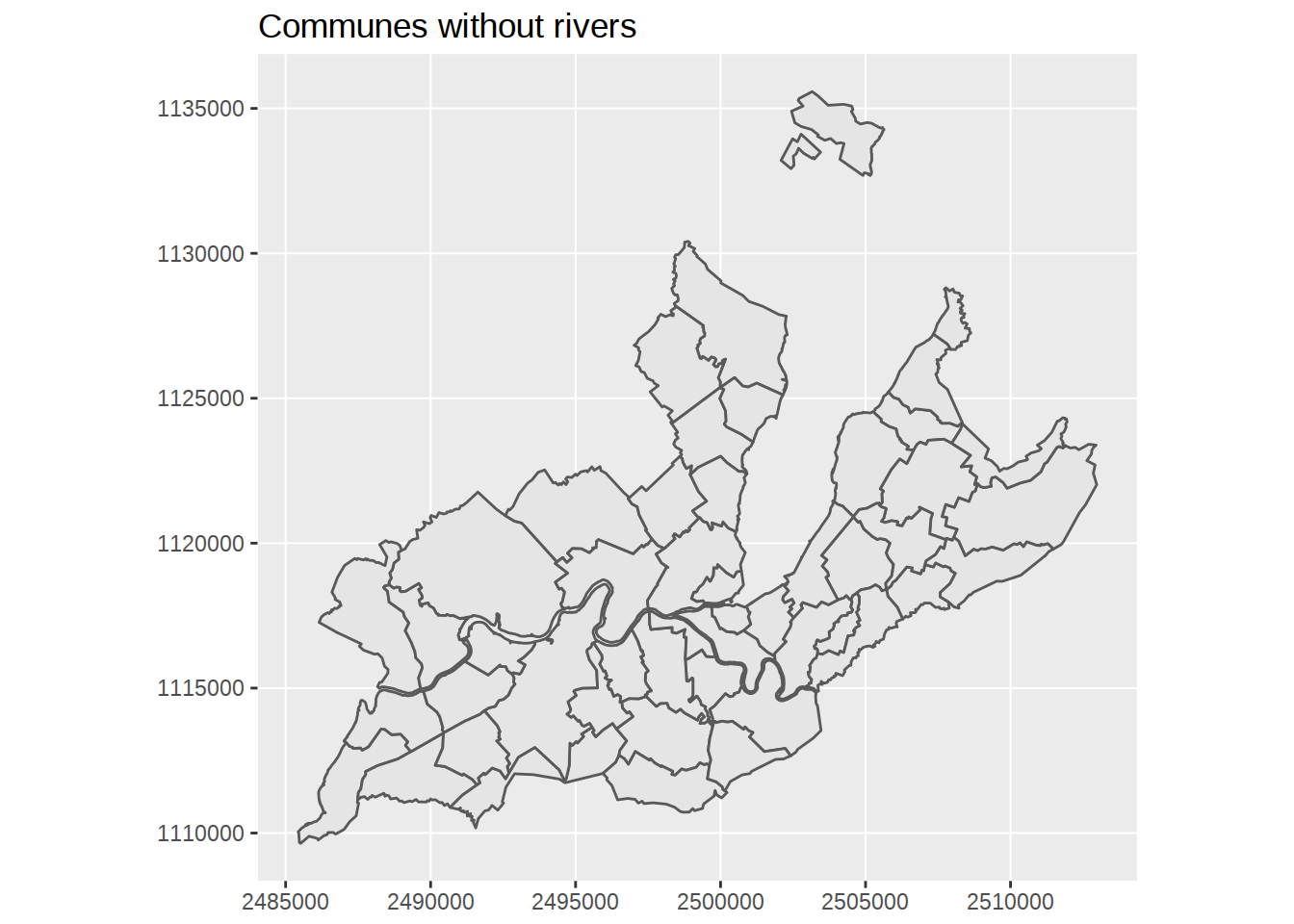

Using these numbers, we can define limits for our map.

ggplot() +
  geom_sf(data=communes_no_water) +
  labs(title="Communes without rivers") +
  # zooming on a smaller region
  coord_sf(xlim=c(2490000,2505000), ylim=c(1115000,1125000))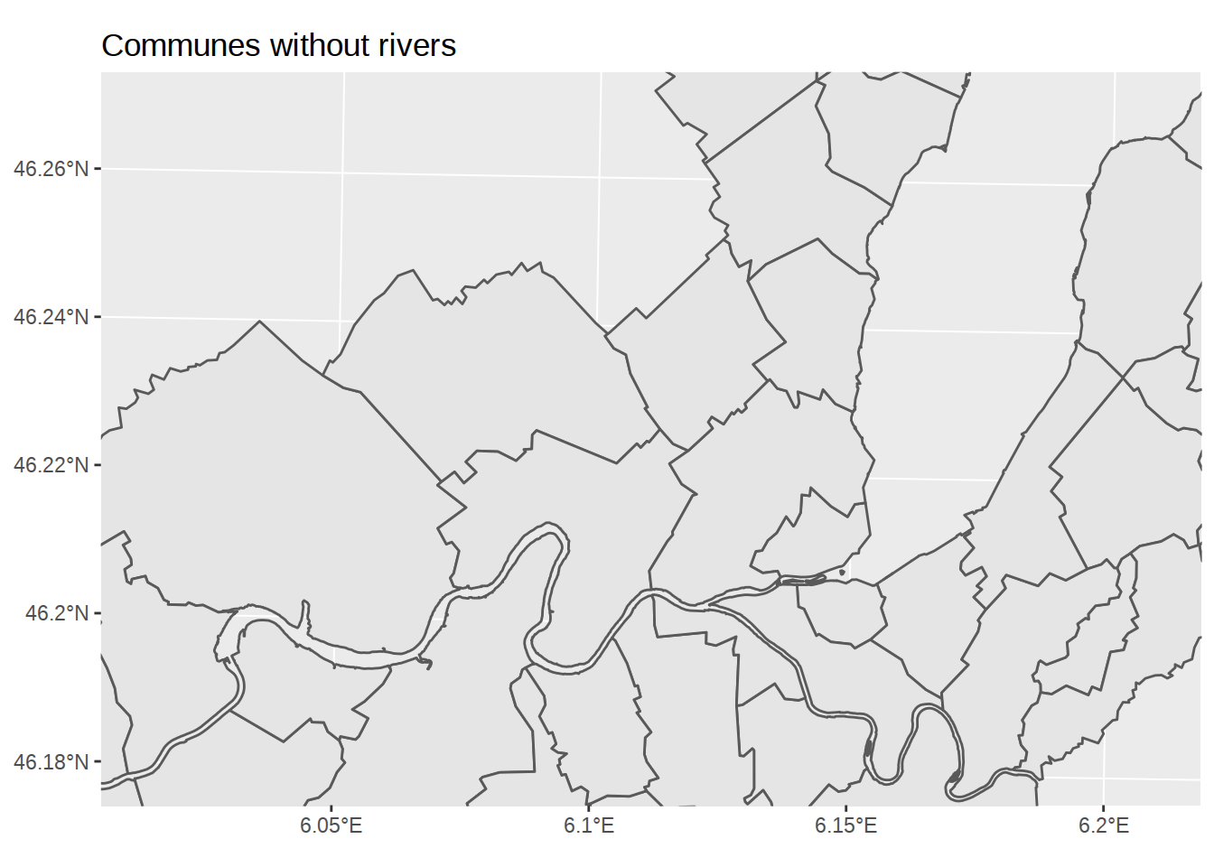

Simplify polygons

The borders are too detailed for the schematic look we are after. To simplify polygons, we can use the rmapshaper package (on Ubuntu, I had to install dependencies libv8-dev and protolite). rmapshaper lets us access the mapshaper javascript library, which provide tools to simplify and modify polygons. We will mainly use the simplify function ms_simplify. Arguments for ms_simplify are described in the vignette.

suppressMessages(library(rmapshaper))
suppressMessages(library(gridExtra))

communes_no_water_simplified <- 
  communes_no_water %>%
    ms_simplify(keep_shapes=T, keep=0.02)

# using grid.arrange from gridExtra
# we can plot the two version side by side
chart_original <-
  ggplot() + 
    geom_sf(data=communes_no_water) +
    labs(title="Original polygons",
         subtitle="No ms_simplify")

chart_simplified <-
  ggplot() + 
    geom_sf(data=communes_no_water_simplified) +
    labs(title="Simplified polygons",
         subtitle="ms_simplify at keep=0.02")

grid.arrange(chart_original, chart_simplified, ncol=2)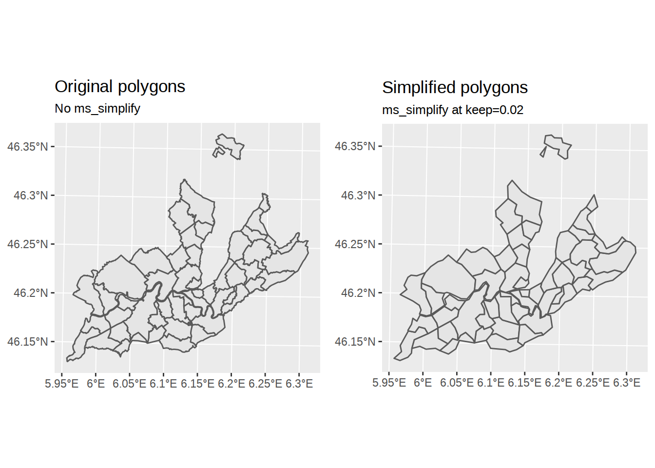

Map land use

The polygons for building, forest and agricultural zones are available here, named ‘AGGLO - ZONES D’AFFECTATION SIMPLIFIEES DE L’AGGLOMERATION FRANCO-VALDO-GENEVOISE’. We can load them with st_read again.

zones <- st_read("../data/AGGLO_ZONE_AFF_SIMPLIFIEE.shp")

## Reading layer `AGGLO_ZONE_AFF_SIMPLIFIEE' from data source `/home/xadam/dev/GitHub/ii_src/content/data/AGGLO_ZONE_AFF_SIMPLIFIEE.shp' using driver `ESRI Shapefile'
## Simple feature collection with 24474 features and 8 fields
## geometry type:  POLYGON
## dimension:      XYZ
## bbox:           xmin: 2465760 ymin: 1089315 xmax: 2531322 ymax: 1155694
## epsg (SRID):    NA
## proj4string:    +proj=somerc +lat_0=46.95240555555556 +lon_0=7.439583333333333 +k_0=1 +x_0=2600000 +y_0=1200000 +ellps=bessel +units=m +no_defs

glimpse(zones)

## Observations: 24,474
## Variables: 9
## $ COMMUNE    <fctr> CROZET, CROZET, CROZET, CROZET, CROZET, CROZET, CR...
## $ LIBFVG     <fctr> Zone de centre village, Zone agricole ou viticole,...
## $ SOURCE     <fctr> PLU, PLU, PLU, PLU, PLU, PLU, PLU, PLU, PLU, PLU, ...
## $ CODECOM    <fctr> 01135, 01135, 01135, 01135, 01135, 01135, 01135, 0...
## $ CODEFVG    <fctr> B, N1, N2, N2, E1y, N2, N2, N2, E1, E1, E1, E1, y,...
## $ CODEURB    <fctr> Ua, Na, N, N, 1AUt, Nh, Nh, Nh, Nt, Ut, Ut, Ut, 2A...
## $ SHAPE_AREA <dbl> 28170.5386, 6904.7535, 2839.2095, 4186.5152, 23454....
## $ SHAPE_LEN  <dbl> 1174.0810, 335.0173, 244.3988, 296.8529, 1367.4976,...
## $ geometry   <simple_feature> POLYGON Z ((2489475.4124 11..., POLYGON ...

Lots of data is contained here. Among the variables, LIBFVG seems to contains the zone types. If we extract the column (encoded as factor), we can use levels to see unique values.

zones$LIBFVG %>%
  levels()

##  [1] "Zone à affectation différée"                       
##  [2] "Zone aéroportuaire"                                
##  [3] "Zone agricole ou viticole"                         
##  [4] "Zone centrale à très forte densité"                
##  [5] "Zone d'activités économiques ou touristiques"      
##  [6] "Zone de centre historique"                         
##  [7] "Zone de centre village"                            
##  [8] "Zone d'équipements publics, sportifs ou de loisirs"
##  [9] "Zone de verdure"                                   
## [10] "Zone future centrale à très forte densité"         
## [11] "Zone future d'activités économiques ou touristiqu" 
## [12] "Zone future de centre village"                     
## [13] "Zone future d'équipements publics, sportifs ou de" 
## [14] "Zone future péricentrale à forte densité"          
## [15] "Zone future péricentrale à moyenne densité"        
## [16] "Zone future périurbaine à faible densité"          
## [17] "Zone liée aux grandes infrastructures de transport"
## [18] "Zone naturelle ou forestière"                      
## [19] "Zone péricentrale à forte densité"                 
## [20] "Zone péricentrale à moyenne densité"               
## [21] "Zone périurbaine à faible densité"

Let’s isolate the building zones and add it as an additional geom_sf layer to our map (grey fill, no borders):

building_zones <- c(
    "Zone périurbaine à faible densité",
    "Zone péricentrale à moyenne densité",
    "Zone péricentrale à forte densité",
    "Zone de centre village",
    "Zone centrale à très forte densité",
    "Zone de centre historique",                         
    "Zone aéroportuaire"
)

ggplot() + 
  geom_sf(data=communes_no_water_simplified) +
  geom_sf(data=zones %>% filter(LIBFVG %in% building_zones),
          fill="grey", color=NA)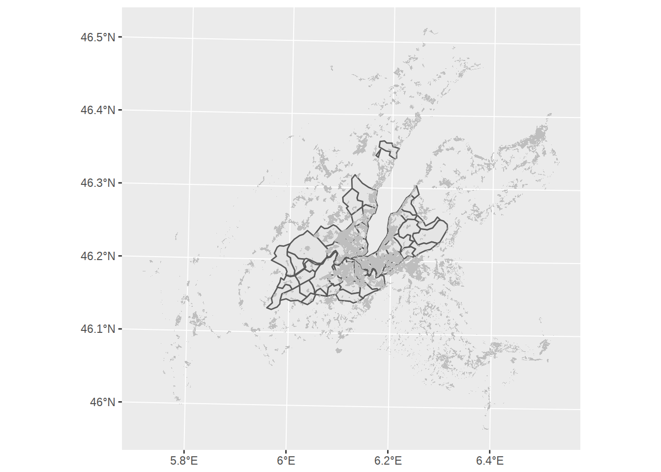

First thing to note: the area covered by the zones polygons is way larger than our little Geneva canton. Previously we used st_difference to find the non-overlapping area. This time, let’s use st_intersection to find overlapping area and “crop” the zones polygons to Geneva area. We will also slightly simplify the polygons with ms_simplify, so they don’t look too detailled compared to our commune borders.

buildings_geneva <-
  zones %>%
   filter(LIBFVG %in% building_zones) %>%
   ms_simplify(keep_shapes = T, keep=0.0001) %>%
   st_intersection(st_union(st_combine(communes_no_water_simplified)))

## Warning: attribute variables are assumed to be spatially constant
## throughout all geometries

ggplot() +
  geom_sf(data=communes_no_water_simplified) +
  geom_sf(data=buildings_geneva, fill="grey", color=NA)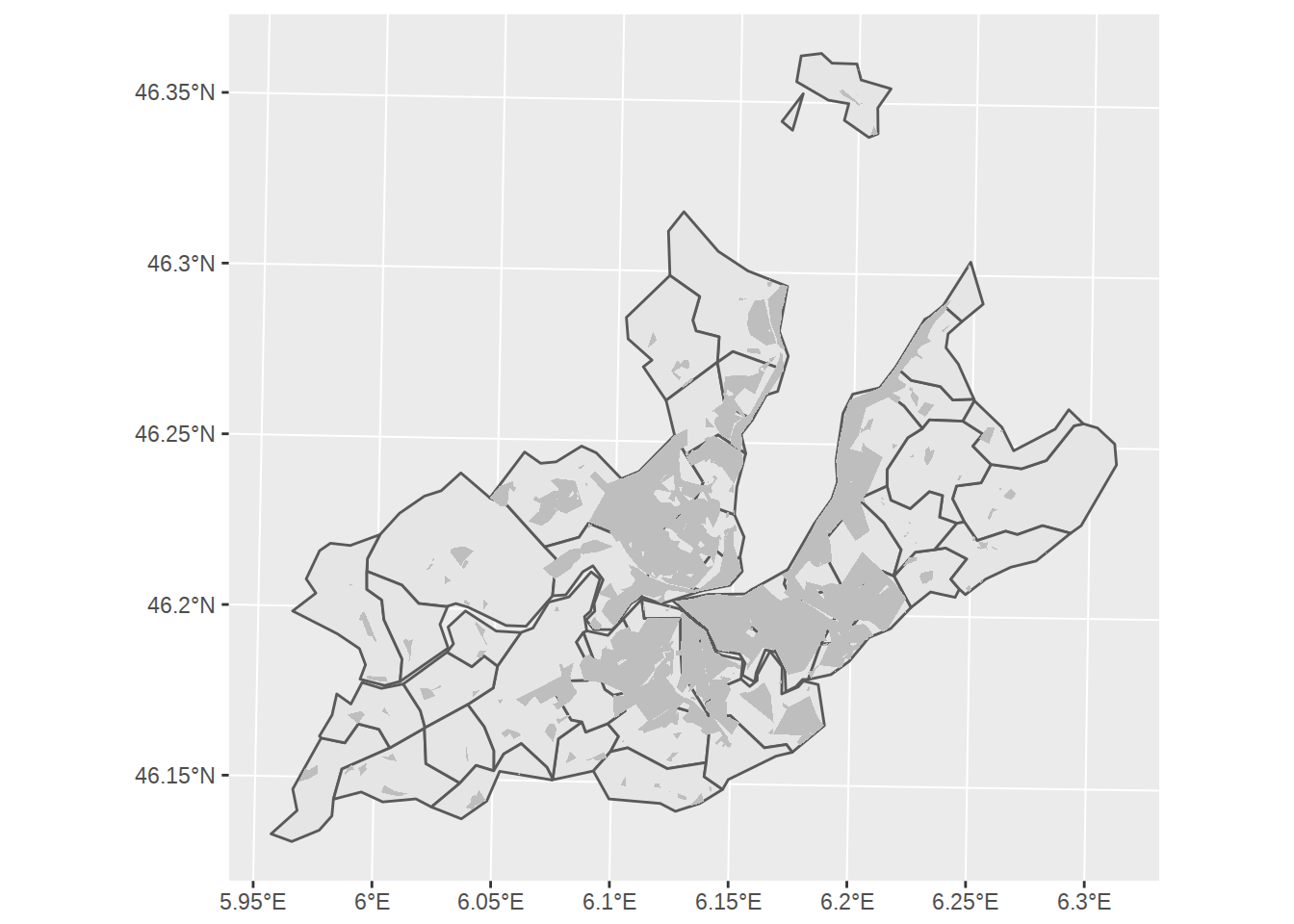

To plot the borders of the communes above the building areas, we can call geom_sf twice rather than once. Remember that ggplot chart work as stack of layers, so each additional geom goes on top of the previous ones.

# Create ggplot
ggplot() +
  # Add polygons for communes, default fill, no border
  geom_sf(data=communes_no_water_simplified, color=NA) +
  # Add polygons for buildings, fill grey, no border
  geom_sf(data=buildings_geneva, fill="grey", color=NA) +
  # Add polygons for communes, no fill, default border
  geom_sf(data=communes_no_water_simplified, fill=NA) +
  labs(title="Geneva communes and buildings")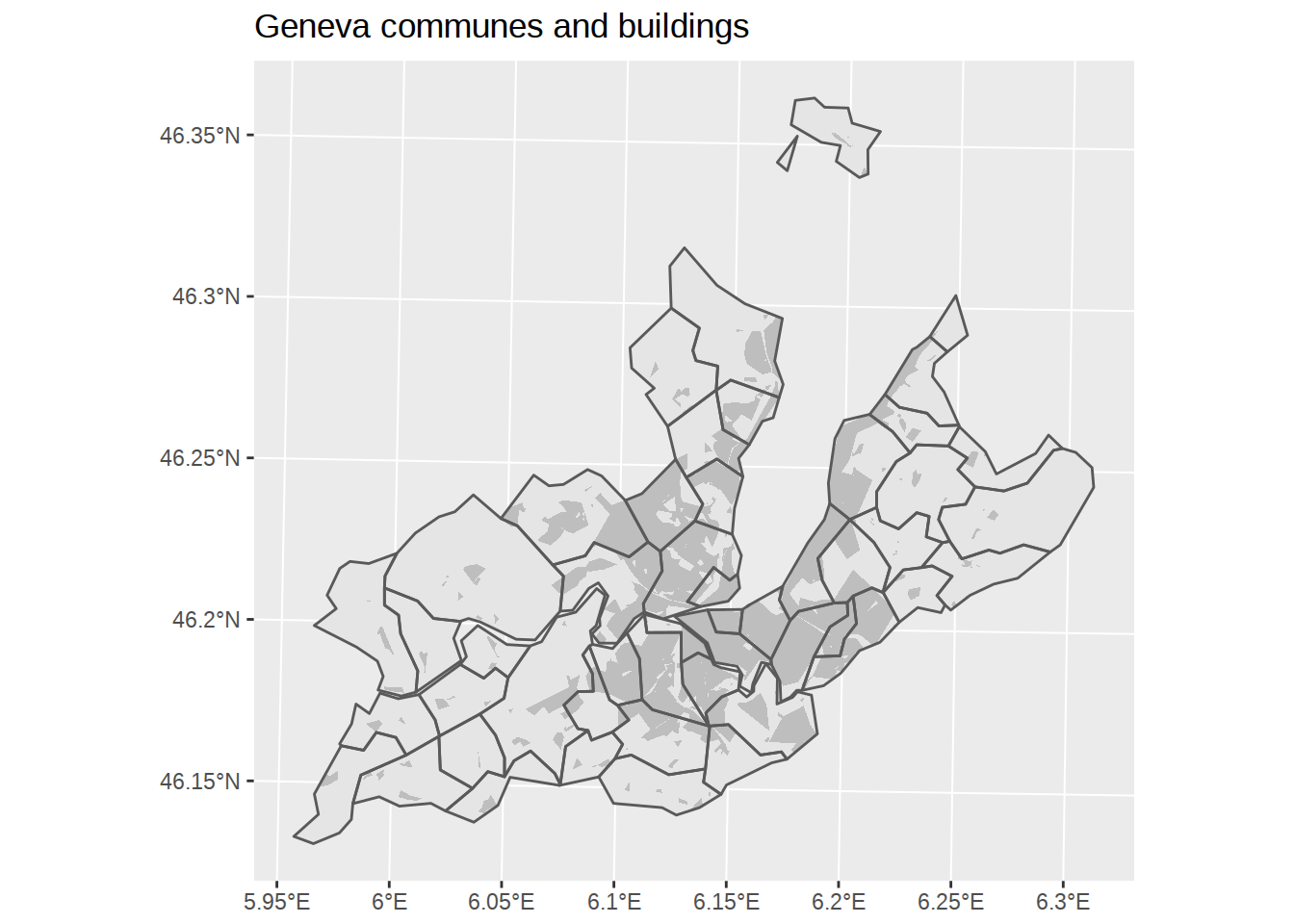

Let’s do the same with the forest areas. When I tried to use st_intersection here, I got TopologyException errors and warnings about Self-intersection. Adding calls to st_make_valid where you get these errors seems to fix the issues.

forest_zones <- c(
    "Zone de verdure"
    ,"Zone naturelle ou forestière"
)

forests_geneva <-
  zones %>%
   filter(LIBFVG %in% forest_zones) %>%
   ms_simplify(keep=0.005) %>%
   st_make_valid() %>%
   st_intersection(st_union(st_combine(communes_no_water_simplified)))

## Warning: attribute variables are assumed to be spatially constant
## throughout all geometries

ggplot() +
  # Add polygons for communes, default fill, no border
  geom_sf(data=communes_no_water_simplified, color=NA) +
  # Add polygons for buildings, fill grey, no border
  geom_sf(data=buildings_geneva, fill="grey", color=NA) +
  # Add polygons for forests, fill grey, no border +
  geom_sf(data=forests_geneva, fill="darkgreen", alpha=0.2, color=NA)+
  # Add polygons borders for communes, no fill, default border
  geom_sf(data=communes_no_water_simplified, fill=NA) +
  labs(title="Geneva communes, buildings and forests")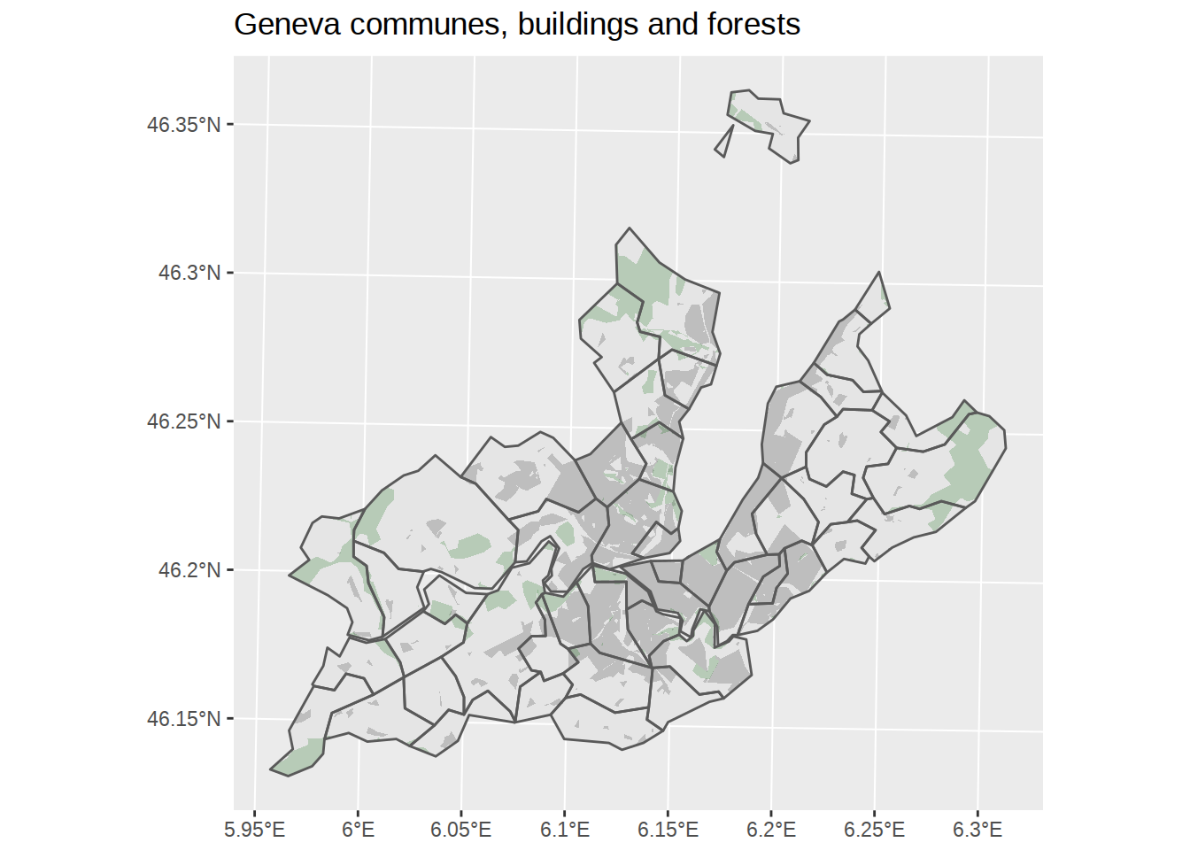

If we got carried away, we could even add the agricultural fields to the map.

fields_geneva <-
  zones %>%
   filter(LIBFVG == "Zone agricole ou viticole") %>%
   ms_simplify(keep=0.005) %>%
   st_make_valid() %>%
   st_intersection(st_union(st_combine(communes_no_water_simplified)))

## Warning: attribute variables are assumed to be spatially constant
## throughout all geometries

ggplot() +
  # Add polygons for communes, default fill, no border
  geom_sf(data=communes_no_water_simplified, color=NA) +
  # Add polygons for forests, fill green, no border +
  geom_sf(data=forests_geneva, fill="darkgreen", alpha=0.2, color=NA)+
  # Add polygons for agricultural area
  geom_sf(data=fields_geneva, fill="yellow", alpha=0.1, color=NA)+
  # Add polygons for buildings, fill grey, no border
  geom_sf(data=buildings_geneva, fill="grey", color=NA) +
  # Add polygons borders for communes, no fill, default border
  geom_sf(data=communes_no_water_simplified, fill=NA) +
  labs(title="Geneva communes, buildings, forests and fields")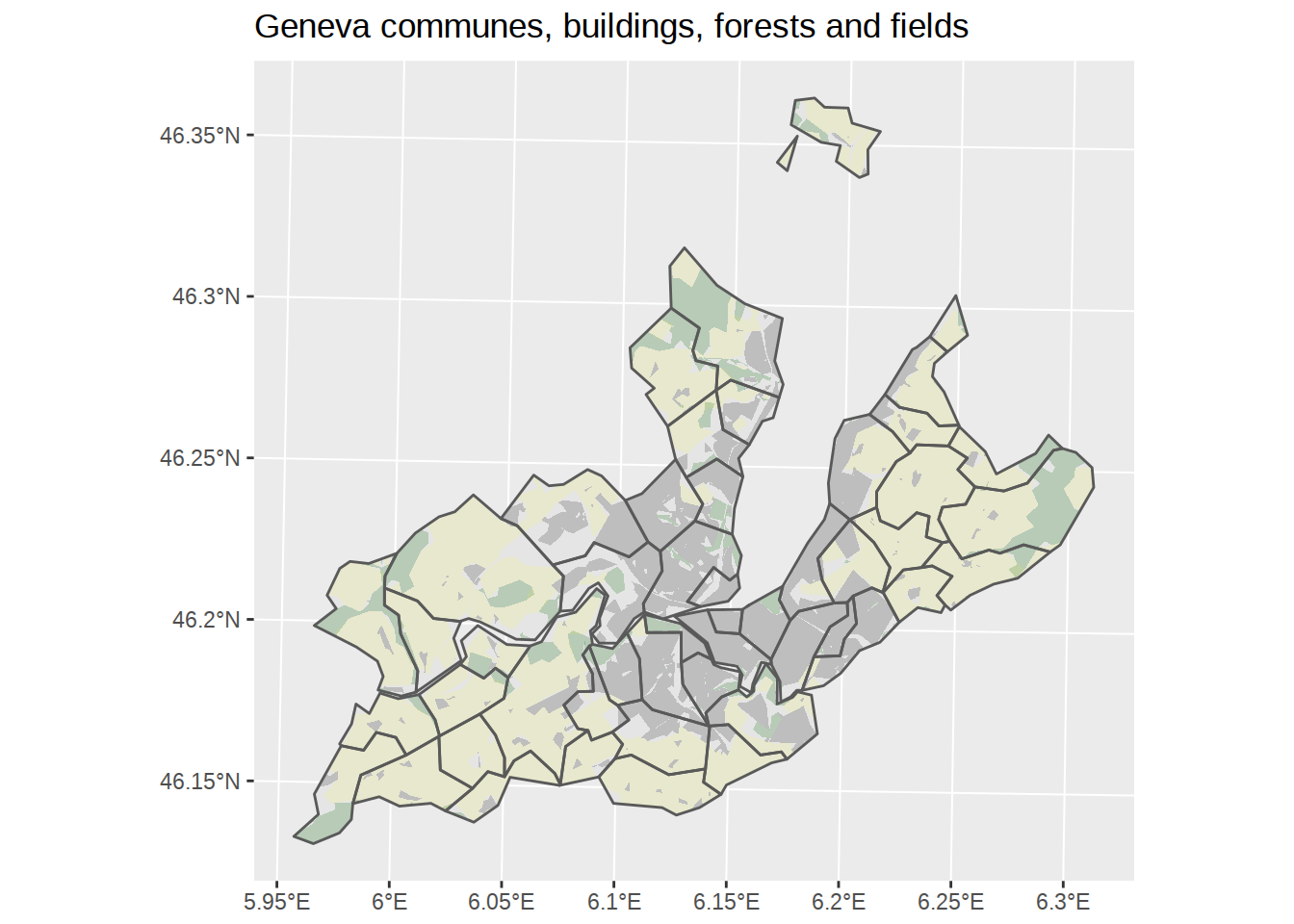

Adding lake and rivers back

What if we decided to add waters back?

ggplot() +
  # Add lake and rivers
  geom_sf(data=waters, fill="blue", color=NA) + 
  # Add polygons for communes, default fill, no border
  geom_sf(data=communes_no_water_simplified, color=NA) +
  # Add polygons for forests, fill green, no border +
  geom_sf(data=forests_geneva, fill="darkgreen", alpha=0.2, color=NA)+
  # Add polygons for agricultural area
  geom_sf(data=fields_geneva, fill="yellow", alpha=0.1, color=NA)+
  # Add polygons for buildings, fill grey, no border
  geom_sf(data=buildings_geneva, fill="grey", color=NA) +
  # Add polygons borders for communes, no fill, default border
  geom_sf(data=communes_no_water_simplified, fill=NA) +
  labs(title="Geneva communes, buildings, forests and fields",
       subtitle="Water is misaligned...")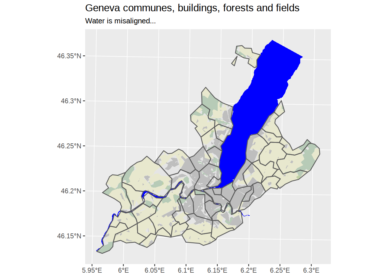

Unfortunately, our water borders cannot match our simplified communes map. Even if we apply exactly the same ms_simplify, it won’t do the trick.

waters_simplified <-
  waters %>%
  ms_simplify(keep_shapes=T, keep=0.02)

ggplot() +
  # Add lake and rivers
  geom_sf(data=waters_simplified, fill="blue", color=NA) + 
  # Add polygons for communes, default fill, no border
  geom_sf(data=communes_no_water_simplified, color=NA) +
  # Add polygons for forests, fill green, no border +
  geom_sf(data=forests_geneva, fill="darkgreen", alpha=0.2, color=NA)+
  # Add polygons for agricultural area
  geom_sf(data=fields_geneva, fill="yellow", alpha=0.1, color=NA)+
  # Add polygons for buildings, fill grey, no border
  geom_sf(data=buildings_geneva, fill="grey", color=NA) +
  # Add polygons borders for communes, no fill, default border
  geom_sf(data=communes_no_water_simplified, fill=NA) +
  labs(title="Geneva communes, buildings, forests and fields",
       subtitle="Water, even simplified, is still misaligned...")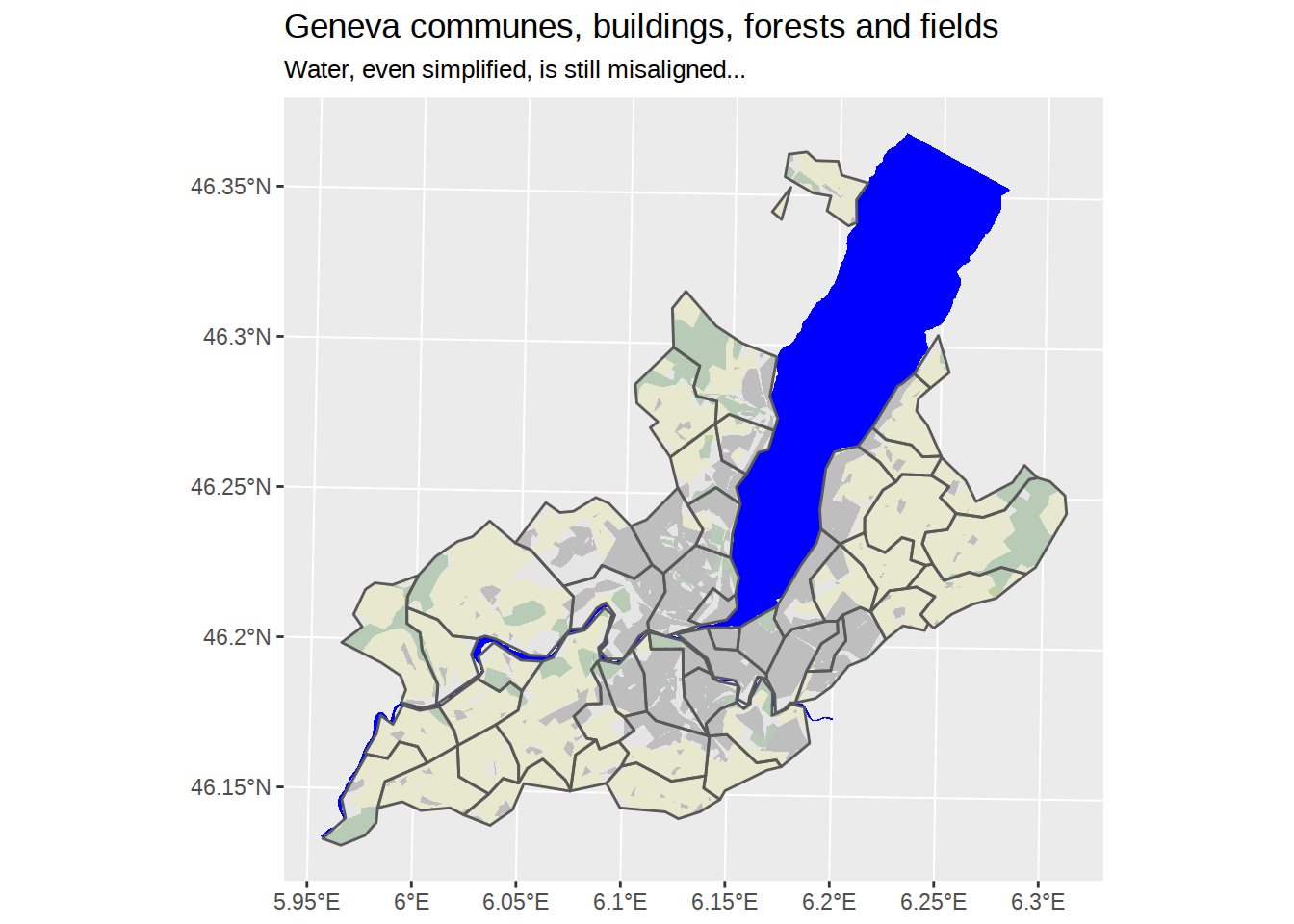

The solution is to merge communes and water into the same sf object before applying ms_simplify.

communes_and_water <- 
  communes %>%
  # remove waters from the original communes
  st_difference(st_union(st_combine(waters))) %>%
  # apply the same columns names so that we
  # can bind waters and communes sf objects
  rename(NOM=COMMUNE) %>%
  select(NOM, SHAPE_AREA, SHAPE_LEN) %>%
  # add the waters polygons
  rbind(waters) %>%
  # simplify
  ms_simplify(keep=0.01) %>%
  st_make_valid()

## Warning: attribute variables are assumed to be spatially constant
## throughout all geometries

ggplot() +
  geom_sf(data=communes_and_water) +
  labs(title="Communes and waters in the same sf",
       subtitle="Simplifed together at 0.01")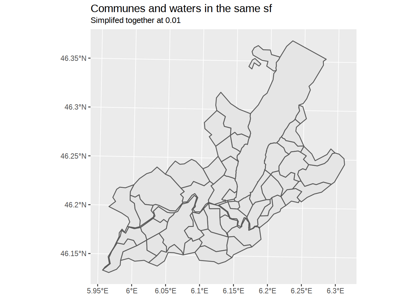

Now that borders are aligned, we can split communes and water again. This makes cropping other sf objects on communes, as well as applying different fill color much easier.

communes_simplified <- 
  communes_and_water %>%
  filter(!(NOM %in% waters$NOM))

waters_simplified <- 
  communes_and_water %>%
  filter(NOM %in% waters$NOM)

buildings_geneva <-
  zones %>%
   filter(LIBFVG %in% building_zones) %>%
   ms_simplify(keep=0.005) %>%
   st_make_valid() %>%
   st_intersection(st_union(st_combine(communes_simplified)))

## Warning: attribute variables are assumed to be spatially constant
## throughout all geometries

forests_geneva <-
  zones %>%
   filter(LIBFVG %in% forest_zones) %>%
   ms_simplify(keep=0.005) %>%
   st_make_valid() %>%
   st_intersection(st_union(st_combine(communes_simplified)))

## Warning: attribute variables are assumed to be spatially constant
## throughout all geometries

fields_geneva <-
  zones %>%
   filter(LIBFVG == "Zone agricole ou viticole") %>%
   ms_simplify(keep=0.005) %>%
   st_make_valid() %>%
   st_intersection(st_union(st_combine(communes_simplified)))

## Warning: attribute variables are assumed to be spatially constant
## throughout all geometries

ggplot() +
  # Add lake and rivers
  geom_sf(data=waters_simplified, fill="lightblue", color=NA) + 
  # Add polygons for communes, default fill, no border
  geom_sf(data=communes_simplified) +
  # Add polygons for forests, fill green, no border +
  geom_sf(data=forests_geneva, fill="darkgreen", alpha=0.2, color=NA)+
  # Add polygons for buildings, fill grey, no border
  geom_sf(data=buildings_geneva, fill="grey", color=NA) +
  # Add polygons for agricultural area
  geom_sf(data=fields_geneva, fill="yellow", alpha=0.1, color=NA)+
  # Add polygons borders for communes, no fill, default border
  geom_sf(data=communes_simplified, fill=NA) +
  labs(title="Geneva communes, buildings and forests")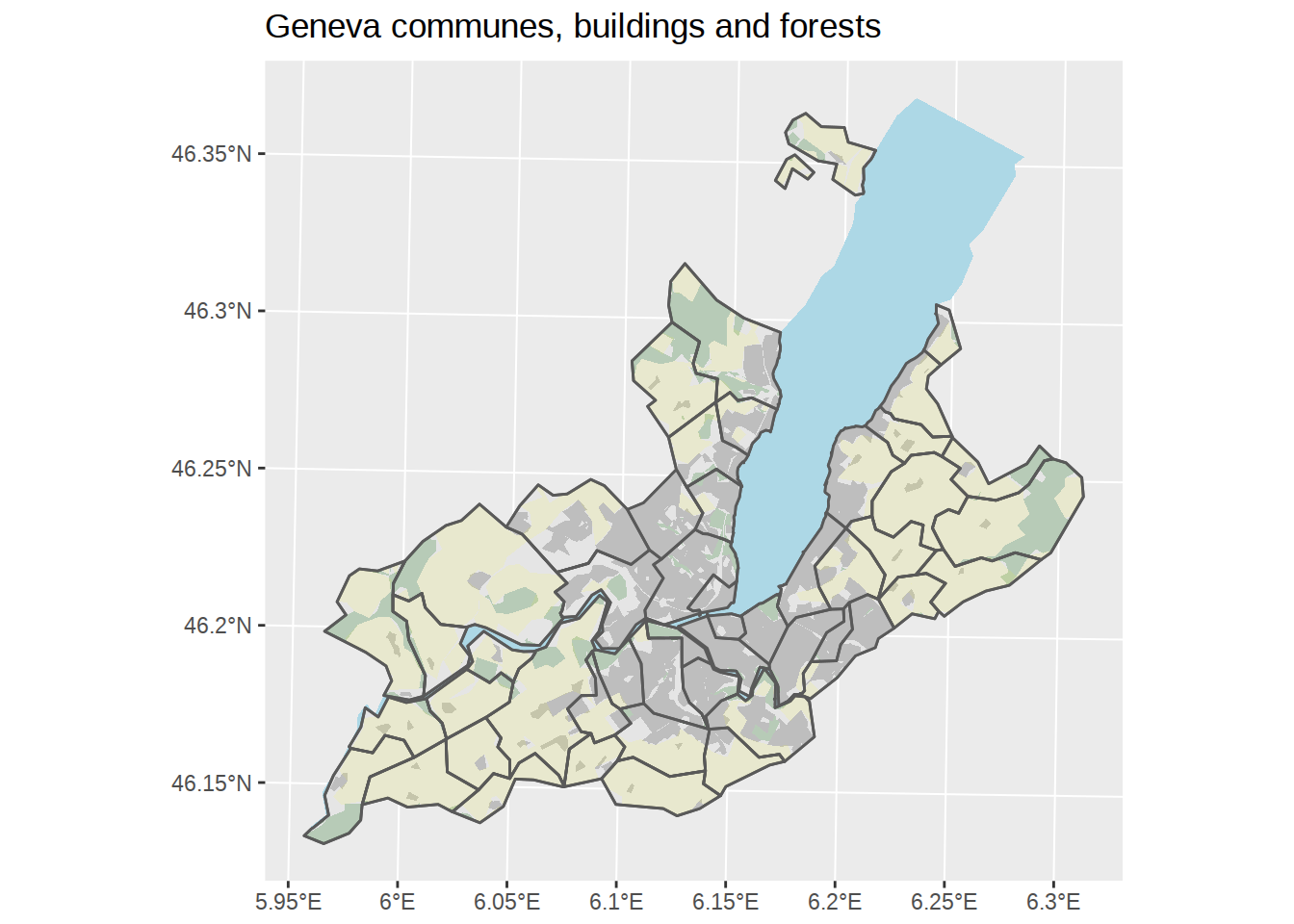

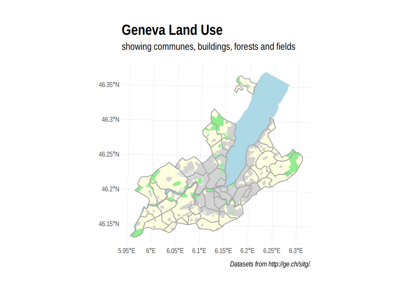
Some more styling

A few final tweaks:

add a caption to mention the source of the data
add fill and border for smoother borders (I see some jagged lines in ubuntu)
apply the ipsum theme from Bob Rudis hrbrthemes

library(hrbrthemes)

ggplot() +
  # Add lake and rivers
  geom_sf(data=waters_simplified, fill="lightblue", color="lightblue") + 
  # Add polygons for communes, default fill, no border
  geom_sf(data=communes_simplified) +
  # Add polygons for forests, fill green, no border +
  geom_sf(data=forests_geneva, fill="lightgreen", color="lightgreen") +
   # Add polygons for agricultural area
  geom_sf(data=fields_geneva, fill="lightyellow", color="lightyellow") +
  # Add polygons for buildings, fill grey, no border
  geom_sf(data=buildings_geneva, fill="lightgrey", color="lightgrey") +
  # Add polygons borders for communes, no fill, default border
  geom_sf(data=communes_simplified, fill=NA, size=0.5, color="darkgrey") +
  labs(title="Geneva Land Use",
       subtitle="showing communes, buildings, forests and fields",
       caption="Datasets from http://ge.ch/sitg/.") +
  theme_ipsum()