Introduction
While reading rweekly past issues, I stumbbled upon a post from Max Humber, explaining how he tried to design a tile grid map / state cartogram for Canada. I had never seen such design and thought that it would be a great fit for Swiss cantons. While browsing the excellent repositories of Bob Rudis, I realised that he had written statebin, a ggplot extension to easily create US state cartogram. This post is my attempt to convert his code to handle Swiss cantons.
In hrbrmstr library, US states are on a 8x12 grid.
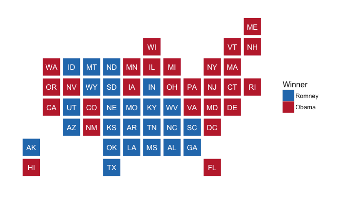
US States mapped with statebins. Source: https://github.com/hrbrmstr/statebins
These coordinates are saved with the full and abbreviated names in a dataframe. The L suffix after the numbers is a way to specify integer.
# Original code from hrbrmstr
# source: https://github.com/hrbrmstr/statebins/blob/master/R/statebins.R
state_coords <- structure(
  list(abbrev = c("AL", "AK", "AZ", "AR", "CA", "CO",
                  "CT", "DC", "DE", "FL", "GA", "HI",
                  "ID", "IL", "IN", "IA", "KS", "KY",
                  "LA", "ME", "MD", "MA", "MI", "MN",
                  "MS", "MO", "MT", "NE", "NV", "NH",
                  "NJ", "NM", "NY", "NC", "ND", "OH",
                  "OK", "OR", "PA", "RI", "SC", "SD",
                  "TN", "TX", "UT", "VT", "VA", "WA",
                  "WV", "WI", "WY", "PR"),
       it = c("Alabama", "Alaska", "Arizona", "Arkansas",
              "California", "Colorado", "Connecticut",
              "District of Columbia", "Delaware", "Florida",
              "Georgia", "Hawaii", "Idaho", "Illinois",
              "Indiana", "Iowa", "Kansas", "Kentucky",
              "Louisiana", "Maine", "Maryland",
              "Massachusetts", "Michigan", "Minnesota",
              "Mississippi", "Missouri", "Montana",
              "Nebraska", "Nevada", "New Hampshire",
              "New Jersey", "New Mexico", "New York",
              "North Carolina", "North Dakota", "Ohio",
              "Oklahoma", "Oregon", "Pennsylvania",
              "Rhode Island", "South Carolina",
              "South Dakota", "Tennessee", "Texas", "Utah",
              "Vermont", "Virginia", "Washington",
              "West Virginia", "Wisconsin", "Wyoming",
              "Puerto Rico"),
       col = c(8L, 1L, 3L, 6L, 2L, 4L, 11L, 10L, 11L, 10L,
               9L, 1L, 3L, 7L, 7L, 6L, 5L, 7L, 6L, 12L,
               10L, 11L, 8L, 6L, 7L, 6L, 4L, 5L, 3L, 12L,
               10L, 4L, 10L, 8L, 5L, 8L, 5L, 2L, 9L, 12L,
               9L, 5L, 7L, 5L, 3L, 11L, 9L, 2L, 8L, 7L, 4L, 12L),
       row = c(7L, 7L, 6L, 6L, 5L, 5L, 4L, 6L, 5L, 8L, 7L,
               8L, 3L, 3L, 4L, 4L, 6L, 5L, 7L, 1L, 5L, 3L,
               3L, 3L, 7L, 5L, 3L, 5L, 4L, 2L, 4L, 6L, 3L,
               6L, 3L, 4L, 7L, 4L, 4L, 4L, 6L, 4L, 6L, 8L,
               5L, 2L, 5L, 3L, 5L, 2L, 4L, 8L)),
  .Names = c("abbrev", "state", "col", "row"),
  class = "data.frame",
  row.names = c(NA, -52L)
)
To sketch the mockup of your tile grid, excel can come to rescue.
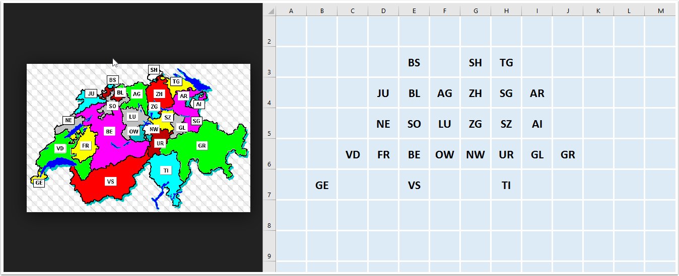
Mock up of Swiss tile grid
This shows that cantons could be represented on a 5x9 grid.
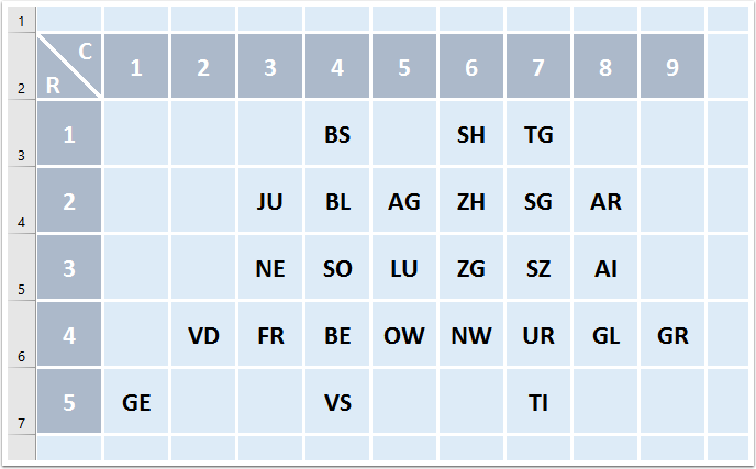
Columns/Rows reference for 5x9 grid
By using the row/column reference of each canton, we can translate this mock up into an object mimicing hrbrmstr data structure (adding the names in each national languages).
canton_coords <- structure(
  list(abbrev = c("AG", "AI", "AR", "BE", "BL", "BS", "FR",
                  "GE", "GL", "GR", "JU", "LU", "NE", "NW",
                  "OW", "SG", "SH", "SO", "SZ", "TG", "TI",
                  "UR", "VD", "VS", "ZG", "ZH"),
       fr_name = c("Argovie", "Appenzell Rhodes-Intérieures",
                   "Appenzell Rhodes-Extérieures", "Berne",
                   "Bâle-Campagne", "Bâle-Ville", "Fribourg",
                   "Genève", "Glaris", "Grisons", "Jura",
                   "Lucerne", "Neuchâtel", "Nidwald", "Obwald",
                   "Saint-Gall", "Schaffhouse", "Soleure", "Schwytz",
                   "Thurgovie", "Tessin", "Uri", "Vaud",
                   "Valais", "Zoug", "Zurich"),
       de_name = c("Aargau", "Appenzell Innerrhoden",
                   "Appenzell Ausserrhoden", "Bern",
                   "Basel-Landschaft", "Basel-Stadt",
                   "Freiburg", "Genf", "Glarus",
                   "Graubünden", "Jura", "Luzern",
                   "Neuenburg", "Nidwalden", "Obwalden",
                   "St. Gallen", "Schaffhausen", "Solothurn",
                   "Schwyz", "Thurgau", "Tessin", "Uri",
                   "Waadt", "Wallis", "Zug", "Zürich"),
       it_name = c("Argovia", "Appenzello Interno",
                   "Appenzello Esterno", "Berna",
                   "Basilea Campagna", "Basilea Città",
                   "Friburgo", "Ginevra", "Glarona",
                   "Grigioni", "Giura", "Lucerna", "Neuchâtel",
                   "Nidvaldo", "Obvaldo", "San Gallo",
                   "Sciaffusa", "Soletta", "Svitto", "Turgovia",
                   "Ticino", "Uri", "Vaud", "Vallese",
                   "Zugo", "Zurigo"),
       ru_name = c("Argovia", "Appenzell Dadens",
                   "Appenzell Dadora", "Berna",
                   "Basilea-Champagna", "Basilea-Citad",
                   "Friburg", "Genevra", "Glaruna",
                   "Grischun", "Giura", "Lucerna", "Neuchâtel",
                   "Sutsilvania", "Sursilvania", "Son Gagl",
                   "Schaffusa", "Soloturn", "Sviz", "Turgovia",
                   "Tessin", "Uri", "Vad", "Vallais",
                   "Zug", "Turitg"),
       col = c(5L,8L,8L,4L,4L,4L,3L,1L,8L,9L,3L,5L,3L,
               6L,5L,7L,6L,4L,7L,7L,7L,7L,2L,4L,6L,6L),
       row = c(2L,3L,2L,4L,2L,1L,4L,5L,4L,4L,2L,3L,3L,
               4L,4L,2L,1L,3L,3L,1L,5L,4L,4L,5L,3L,2L)),
  .Names = c("abbrev", "fr_name", "de_name",
             "it_name", "ru_name", "col", "row"),
  class = "data.frame",
  row.names = c(NA, -26L)
)
Using the same data structure as the one designed for statebin, it is easy to reuse the same ggplot code and only apply slight modifications (like a theme from the same hrbrmstr).
suppressMessages(library(ggplot2))
suppressMessages(library(RColorBrewer))
suppressMessages(library(hrbrthemes))

cantonbins <- function(canton_data, canton_col="abbrev", value_col="value",
                     text_color="black", font_size=3,
                     canton_border_col="white", labels=1:5,
                     brewer_pal="PuBu", plot_title="",
                     plot_subtitle="", plot_caption="") {

  # Reformat canton_data into a data frame without factors
  # and merge with canton_coords on abbrev key
  canton_data <- data.frame(canton_data, stringsAsFactors=FALSE)
  merge.x <- "abbrev"
  ct.dat <- merge(canton_coords, canton_data,
                  by.x=merge.x, by.y=canton_col, all.y=TRUE)

  # Create tile plot
  gg <- ggplot(ct.dat, aes_string(x="col", y="row", label="abbrev"))
  gg <- gg + geom_tile(aes_string(fill=value_col))
  gg <- gg + geom_tile(color=canton_border_col, aes_string(fill=value_col),
                       size=2, show.legend =FALSE)
  gg <- gg + geom_text(color=text_color, size=font_size)

  # Add title
  gg <- gg + labs(title=plot_title, subtitle=plot_subtitle,
                  caption=plot_caption)

  # Set scales and coordinates system
  gg <- gg + scale_y_reverse()
  gg <- gg + scale_fill_gradientn(colours = brewer.pal(6, brewer_pal))
  gg <- gg + coord_equal()

  # Set minimal theme and remove axis titles, border, grid,
  # background, axis ticks and axis text
  gg <- gg + theme_ipsum_rc()
  gg <- gg + labs(x=NULL, y=NULL)
  gg <- gg + theme(panel.border=element_blank())
  gg <- gg + theme(panel.grid=element_blank())
  gg <- gg + theme(panel.background=element_blank())
  gg <- gg + theme(axis.ticks=element_blank())
  gg <- gg + theme(axis.text=element_blank())

  return(gg)
}
To test the function, let’s scrape a table from wikipedia containing the population per cantons. By inspecting the wikipedia code, you can see that the table has the class: wikitable. It can be extracted (with the help of rvest) and converted into a usable dataframe (using dplyr). The only modification are:
- renaming the
Population[Note 2]column to something simpler - converting the numbers stored as strings to numeric after removing their thousands “,”
- remove the total row for Switzerland (
Code != "CH") - selecting the columns of interest
suppressMessages(library(rvest))
suppressMessages(library(dplyr))
suppressMessages(library(stringr))
suppressMessages(library(DT))

url <- "https://en.wikipedia.org/wiki/Cantons_of_Switzerland"
density <- url %>%
  read_html() %>%
  html_node(xpath='//table[contains(@class,"wikitable")]') %>%
  html_table() %>%
  rename(Population=`Population[Note 2]`) %>%
  # Remove comma and notes reference (digit between brackets)
  mutate(Population=as.numeric(
    stringr::str_replace_all(
      Population, "(,|(\\[[:digit:]*\\]))", ""))) %>%
  filter(Code != "CH") %>%
  select(Code, Canton, Population)

DT::datatable(
  density,
  options = list(pageLength = 5, dom = 'tpi'),
  rownames = FALSE,
  caption = "Table 1 : Subset of wikipedia data for cantons.")
We can now try the cantonbins function.
cantonbins(density, canton_col="Code", value_col="Population",
           plot_title="Population size in Swiss Cantons",
           plot_subtitle = paste0("Source: ", url))
There is a lot more we can do with Cartograms and, in a future post, I hope to release a full fork of statebin so that you can easily install it from Github.